Continuum Subtraction

Scripts for Step 4 - Prepare the lines:

step4_prepare_lines.py # main script
step4_detour.py # for phase alignment
dictionary_data.py # loads data_dict
step1_utils.py # loads multiple functions
analysisUtils (analysis_scripts/) # for channel strings

Continuum Subtraction#

We perform continuum subtraction in uv-space with CASA task uvcontsub.

Channels used to fit the continuum are the inverse of those used to flag the spectral lines in Pseudo-continuum Measurement Sets. We again use the DSHARP function get_flagchannels (reductions_utils.py) using the same velocity ranges selected in Step 1, and then “flip” them using the analysisUtils function invertChannelRanges:

Relevant lines in step4_prepare_lines.py

flagchannels_string = get_flagchannels(ms_file          = inputvis,
                                       ms_dict          = data_dict[EB],
                                       velocity_range   = data_dict[EB]['velocity_ranges'])
fitspw = au.invertChannelRanges(flagchannels_string, vis=inputvis)

Relevant lines in dictionary_data.py

velocity_ranges = np.array([np.array([ddisk.disk_dict['v_sys']-3., ddisk.disk_dict['v_sys']+3.]),
                            np.array([ddisk.disk_dict['v_sys']-4., ddisk.disk_dict['v_sys']+4.]),
                            np.array([ddisk.disk_dict['v_sys']-6., ddisk.disk_dict['v_sys']+6.]),
                            np.array([ddisk.disk_dict['v_sys']-10., ddisk.disk_dict['v_sys']+10.])])

Here are the resulting channels in each spectral window to be used by uvcontsub to fit the continuum, formatted as the necessary strings:

Flagchannels input string for SB_EB1: '1:517~589,       2:504~600,       3:961~1251,        4:556~1059'
                              fitspw:  1:0~516;590~959, 2:0~503;601~959, 3:0~960;1252~1919, 4:0~555;1060~1919
Flagchannels input string for SB_EB2: '1:517~589,       2:504~600,       3:962~1251,        4:554~1058'
                              fitspw:  1:0~516;590~959, 2:0~503;601~959, 3:0~961;1252~1919, 4:0~553;1059~1919
Flagchannels input string for LB_EB1: '1:516~589,       2:504~600,       3:960~1249,        4:553~1057'
                              fitspw:  1:0~515;590~959, 2:0~503;601~959, 3:0~959;1250~1919, 4:0~552;1058~1919
Flagchannels input string for LB_EB2: '1:517~589,       2:504~600,       3:960~1249,        4:553~1057'
                              fitspw:  1:0~516;590~959, 2:0~503;601~959, 3:0~959;1250~1919, 4:0~552;1058~1919
Flagchannels input string for LB_EB3: '1:517~589,       2:505~601,       3:960~1249,        4:553~1057'
                              fitspw:  1:0~516;590~959, 2:0~504;602~959, 3:0~959;1250~1919, 4:0~552;1058~1919
Flagchannels input string for LB_EB4: '1:516~589,       2:504~600,       3:960~1249,        4:553~1057'
                              fitspw:  1:0~515;590~959, 2:0~503;601~959, 3:0~959;1250~1919, 4:0~552;1058~1919
Flagchannels input string for LB_EB5: '1:516~588,       2:504~600,       3:960~1250,        4:553~1057'
                              fitspw:  1:0~515;589~959, 2:0~503;601~959, 3:0~959;1251~1919, 4:0~552;1058~1919
Flagchannels input string for LB_EB6: '1:517~589,       2:505~601,       3:960~1249,        4:553~1057'
                              fitspw:  1:0~516;590~959, 2:0~504;602~959, 3:0~959;1250~1919, 4:0~552;1058~1919

The call to uvcontsub will re-index our line spectral windows.

Relevant lines in step4_prepare_lines.py

for EB in data_dict['EBs']:            # this takes 1hr10min per LB EB
    inputvis            = data_dict['NRAO_path']+data_dict[EB]['_initlines_selfcal.ms']
    outputvis           = data_dict['NRAO_path']+data_dict[EB]['_initlines_selfcal.ms.contsub']
    spw                 = '1, 2, 3, 4' # only line spws; they will be renumbered 0,1,2,3
    combine             = ''           # break at scan, field, and spw
    fitorder            = 1            # order of polynomial fit; default is 0; DSHARP uses 1 so we copy them
    solint              = 'int'        # Timescale for per-baseline fit. default (recommended): ‘int’, i.e. no time averaging, do a fit for each integration and let the noisy fits average out in the image.continuum
    excludechans        = False        # the channels in fitspw will be used to fit the continuum
    want_cont           = False        # we don't need another ms to hold the continuum estimate

    os.system('rm -rf ' + outputvis)
    uvcontsub(vis=inputvis, spw=spw, combine=combine, fitorder=fitorder,
                       solint=solint, excludechans=excludechans, want_cont=want_cont,
                       fitspw=fitspw)
    listobs(vis=outputvis, listfile=outputvis+'.listobs.txt')

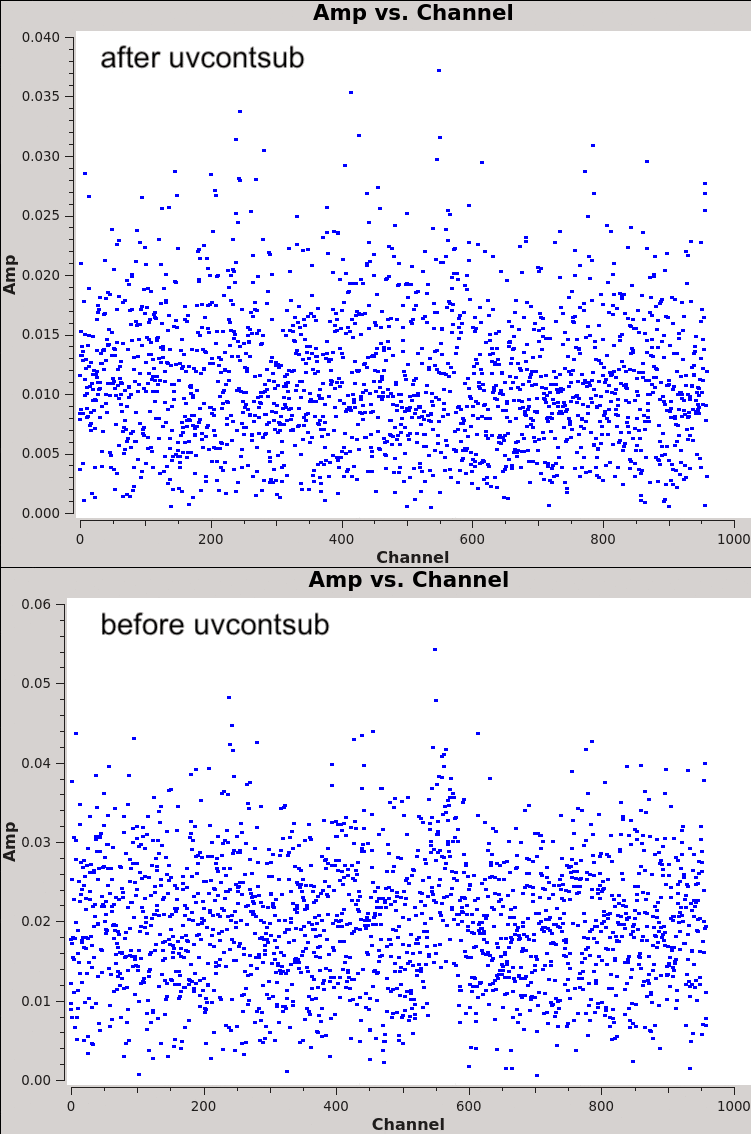
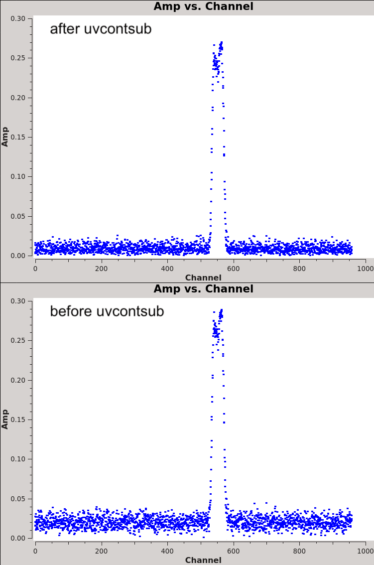
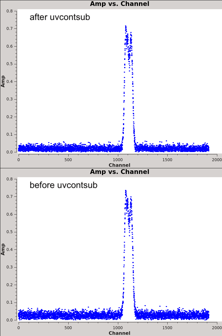
Here is the before-and-after, for SB EB 1, for spectral windows SO, C¹⁸O, ¹³CO, and ¹²CO (left to right):

Example before/after continuum subtraction (SB EB 1)

Amplitude vs. channel, before and after continuum subtraction. These plots were made with avgtime='1e8', avgscan=True and avgbaseline=True.