Warning
This page is a journal of experiments and initial approaches to the line imaging. It is intended to serve as a blog more than anything else. I’ve kept a record of these experiments on the off chance that some aspects could be helpful to others in some niche cases. The imaging script corresponding to these initial experiments is image_lines.py.
The main take-aways from these initial (unsuccessful) approaches are summarized on the next page, Summary of Challenges Motivating the Adopted Imaging Strategy. The final approach taken for the published line images is described on the last page, Adopted Imaging Strategy. The corresponding imaging script is major_image_lines.py.
Journal of Challenges and Initial Experiments#
Over-arching Challenge: Masking for Clean#
Cleaning and Masking
The tclean task gives the user the option to indicate where in the image to clean. The idea is that, inside the mask, the emission should be real (and therefore included in our model), and outside the mask, any emission should just be noise (and therefore excluded from the model).
For protoplanetary disks, we have some knowledge of where we expect their emission to appear throughout the channels, because we expect the bulk of the disk to be rotating Keplerian. Rich Teague therefore wrote his keplerian_mask package, which is widely used for masking when making clean images of disks.
Problem: Appropriate clean mask for AB Aur?
Can we use a Keplerian mask for AB Aur? That would be super convenient, but if we look at the dirty images of 12CO, 13CO, and even C18O, the emission is clearly highly non-Keplerian. We therefore need to explore other options for masking.
Possible solutions: Ways to make clean masks for AB Aur
Ryan foresaw our need to explore other options for masking and gave a couple possible ideas:
Use manually drawn masks. This involves spending (potentially a lot of) time upfront to define the masks by hand, but then you have them and can reuse them continuously. MAPS did this for their 12CO images (Rich Teague took the time to draw the masks for 12CO by hand, and then they used Keplerian masks for everything else). Here’s some central channels of Rich’s custom CO mask for GM Aur:
Use a Keplerian mask to define a “starting” mask, and then edit it by hand from there. In other words, save time by not drawing a mask from scratch.
Use automasking (‘auto-multithresh’). This works well but is slow. Auto-multithresh is flexible; it draws an initial mask, and then updates it (grows it) during subsequent clean cycles. Here the time investment is re-spent every time you clean.
Take a dirty image, clean it a little bit, and define a mask based on the regions where the emission is over some threshold value.
Bounce back and forth. There’s no good recipe that works for everything. Try a couple different things, see what works, and go with that.
More possible solutions: Huang+2021 (MAPS) approach to clean mask for GM Aur
Can we find examples or guidance in the literature for situations like our own?
Huang et al. (2021, MAPS) seem to have had a similar issue of non-Keplerian emission with their re-imaging of GM Aur in 12CO, and did something different to the MAPS fiducial imaging pipeline (Czekala et al. 2021). Instead of Rich’s custom CO mask, they used auto-multithresh to automatically generate masks in tclean on the fly, using some input threshold parameters. The relevant sentences are (Sec. 2.1):
We applied the multiscale CLEAN algorithm (Cornwell 2008) with scales of
[0, 0.4, 1", 2"]. Since 12CO was also reobserved at higher spectral resolution than the other lines, we reimaged 12CO with channel widths of 0.1 km/s for better recovery of the kinematic details. Due to the irregular emission morphology, we used CASA’s auto-multithresh algorithm (Kepley et al. 2020) to draw the CLEAN mask. The auto-multithresh algorithm searches the cube for significant emission, beginning with a relatively conservative mask and then expanding to encompass more emission during subsequent major cycles. The mask was initialized with full coverage of the primary beam from 5.2–6.4 km/s, where the emission is the broadest, because auto-multithresh algorithm does not readily mask diffuse emission. After some experimentation, the following auto-multithresh parameters were selected:sidelobethreshold = 3.0,noisethreshold = 4.0,lownoisethreshold = 1.5, andminbeamfrac = 0.3. The CLEAN threshold was set to 5 mJy, corresponding to ~3× the rms of line-free channels in the dirty image. – (Huang et al. 2021)
1st round of imaging experiments#
1st imaging approach taken: Masking emission with auto-multithresh and the Huang et al. (2021) parameters
The sidelobethreshold and noisethreshold parameters Huang et al. (2021) used are both lower (by 1.0) than the defaults in the “Table of Standard Salues: 12m (long) b75>300m” (specified in the Automasking Guide). Effectively, lowering these two parameters makes auto-multithresh “more flexible”, allowing the mask to grow a little more into lower signal areas than the default values allow.
Results: Auto-multithresh fails to capture extended/diffuse extended emission. There is emission that is not being included in the model.
I found that even with lowered sidelobethreshold and noisethreshold parameters, auto-multithresh fails to capture extended/diffuse extended emission in 12CO and 13CO cubes. We can see this in the movies below. The problem is most clear to see in the rightmost panels, which show the residuals (what’s left after tclean has finished). In all movies, the white contours are the “final” auto-multithresh mask (i.e., the mask used on the last cleaning cycle – all previous cycles’ masks would have been less extended, since the mask can only grow between cycles). There are strong residuals outside the mask. This means there is emission that is not being included in the model. This is problematic because:
If we use JvM-corrected images, the uncaptured emission will be downscaled (by the factor epsilon).
The cleaning will not actually reach the threshold, meaning the final images will be more shallowly cleaned than we specified. (It’s a self-closing loop: tclean/auto-multithresh uses the unmasked regions to estimate the noise left in the residuals, so if it’s estimating the noise using the regions with diffuse emission, it will think it’s reached the threshold sooner than it has, and therefore stop cleaning, and stop growing the mask.)
2nd round of imaging experiments#
2nd imaging approach taken: Masking emission with auto-multithresh and the Huang et al. (2021) parameters, but kickstarting auto-multithresh with a broad mask
Referring back to Huang et al. (2021), we see they had a solution to the problem of auto-multithresh not masking diffuse emission:
The mask was initialized with full coverage of the primary beam from 5.2–6.4 km/s, where the emission is the broadest, because auto-multithresh algorithm does not readily mask diffuse emission. – (Huang et al. 2021)
I then discovered that getting auto-multithresh to actually use a pre-defined mask is non-trivial. The Automasking Guide provides some information at the bottom of the page, under the section titled Advanced Use Case - Merging User Masks with Automasking. So, this seems to be a bit niche, but at least it is a known issue.
Kickstarting auto-multithresh with a broad mask involves:
Make the (initial, broad) mask that you want auto-multithresh to start with. [For this I actually took Rich Teague’s keplerian_mask code and modified it to give me a broad ellipse at all channels within a range I defined. In hindsight there are probably simpler ways to do this, but at the time I had no easier ideas.]
Do one initial round of cleaning with the (initial, broad) mask, and without auto-multithresh. For this round I set
niter=cycleniter=1(it’s important thatniter=cycleniter, and both=1simply so that the least amount of cleaning happens).Restart
tclean, now with auto-multithresh turned on, and givetcleaninstructions to pick up where the initial clean left off.
For making the (initial, broad) mask, my first approach was to take the sentence “The mask was initialized with full coverage of the primary beam from 5.2–6.4 km/s, where the emission is the broadest” (Huang et al. 2021) to heart, and initialize the broad mask only in the channels where emission is broadest (and therefore have no mask, for this initial round of tclean, in the other channels, trusting that auto-multithresh will make its own). I chose the channel ranges based on where auto-multithresh had started failing to capture the emission in the “1st round of imaging experiments”.
Results: It works, but the broad initial mask should encompass an even larger range of channels
This seems to have worked well. Auto-multithresh did pick up the broad initial mask and take it from there. It won’t shrink its mask in subsequent iterations, so we’re stuck with the broad mask. But, this approach does seem to capture the diffuse emission in the clean image yield relatively even residuals inside the mask.
Room for improvement: The broad initial mask should encompass an even larger range of channels. In the residuals movie (middle), there are still some residuals outside the auto-multithresh mask (e.g. 4.8 km/s, 6.942 km/s). If we look at the model (bottom panel), we can see the multi-scale deconvolver putting many small-Gaussians right up against the edge of the mask, trying to encompass the emission that extends over the sides. This suggests we just need to increase the channel range of the broad initial mask, to include bluer and redder channels.
3rd round of imaging experiments#
3rd imaging approach taken: Masking emission with auto-multithresh and the Huang et al. (2021) parameters, but kickstarting auto-multithresh with a broad mask, now over a wider range of channels
Here I did the same thing as the 2nd round of imaging experiments, but initializing the broad mask to cover bluer and redder channels.
Results: Significant residuals left inside the mask, cleaning is discontinuous in velocity space, tail channels not cleaned at all (“channel dropout”)
This seems to have not worked as well. The 3 problems I see are:
The residuals within the mask after cleaning are not of the same magnitude as the “noise” outside the mask. There are significant residuals inside the mask that are spatially uneven. [This can be seen in the residual movies below.]
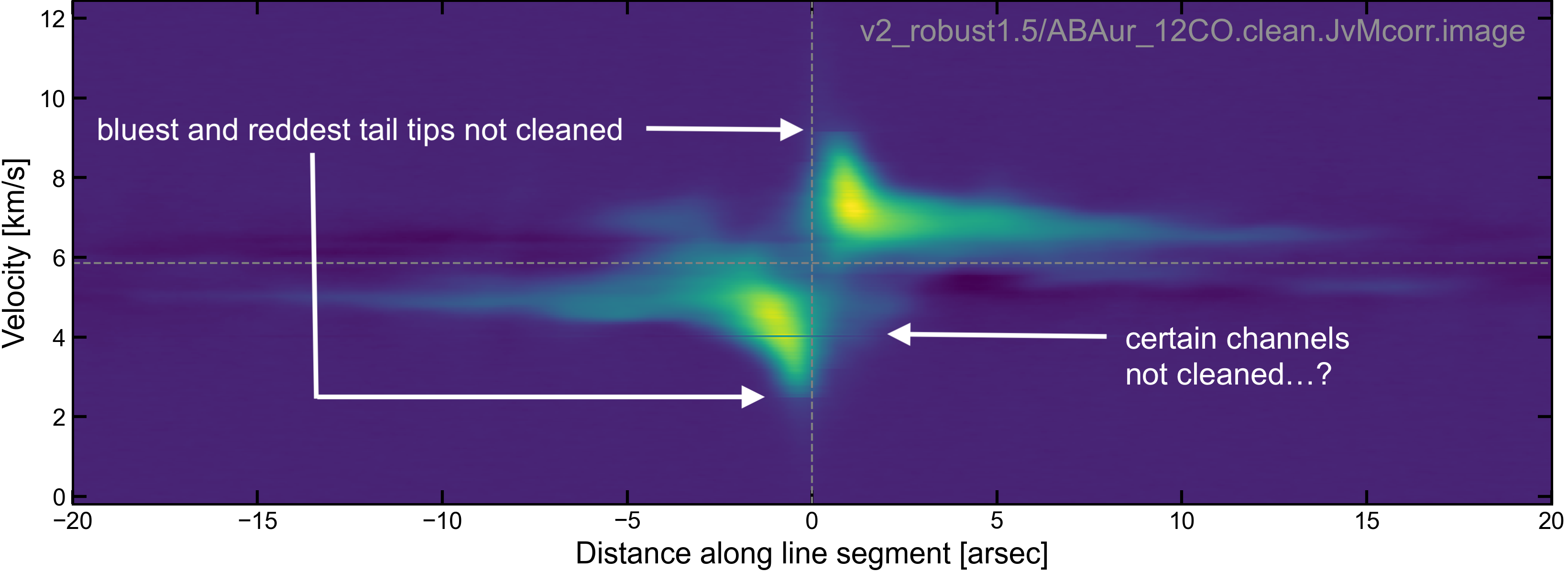
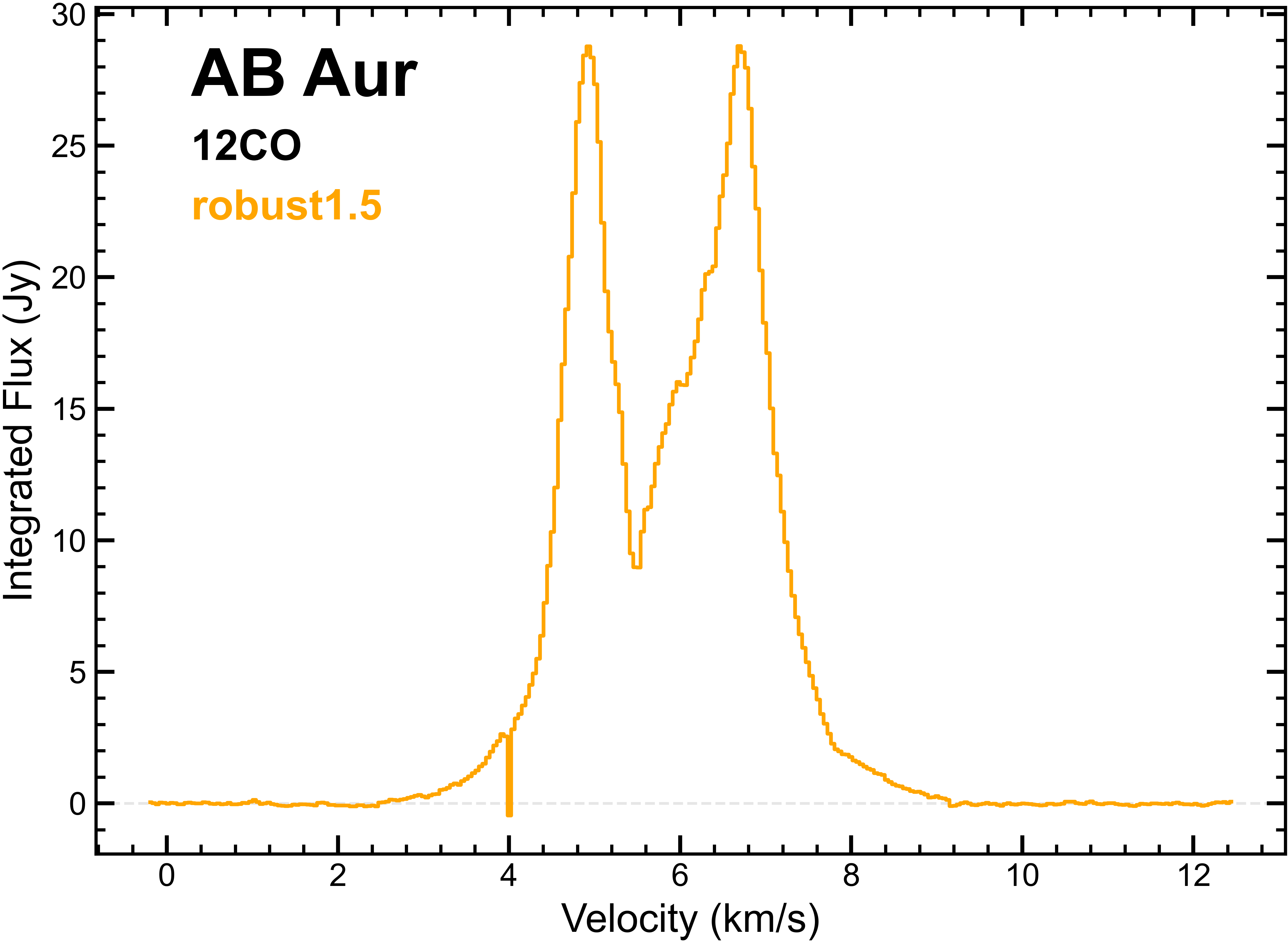
The cleaning is uneven in velocity space. Some channels have extremely large residuals in a discontinuous way from other channels. [A good example of this is at 4.002 km/s in 12CO.]
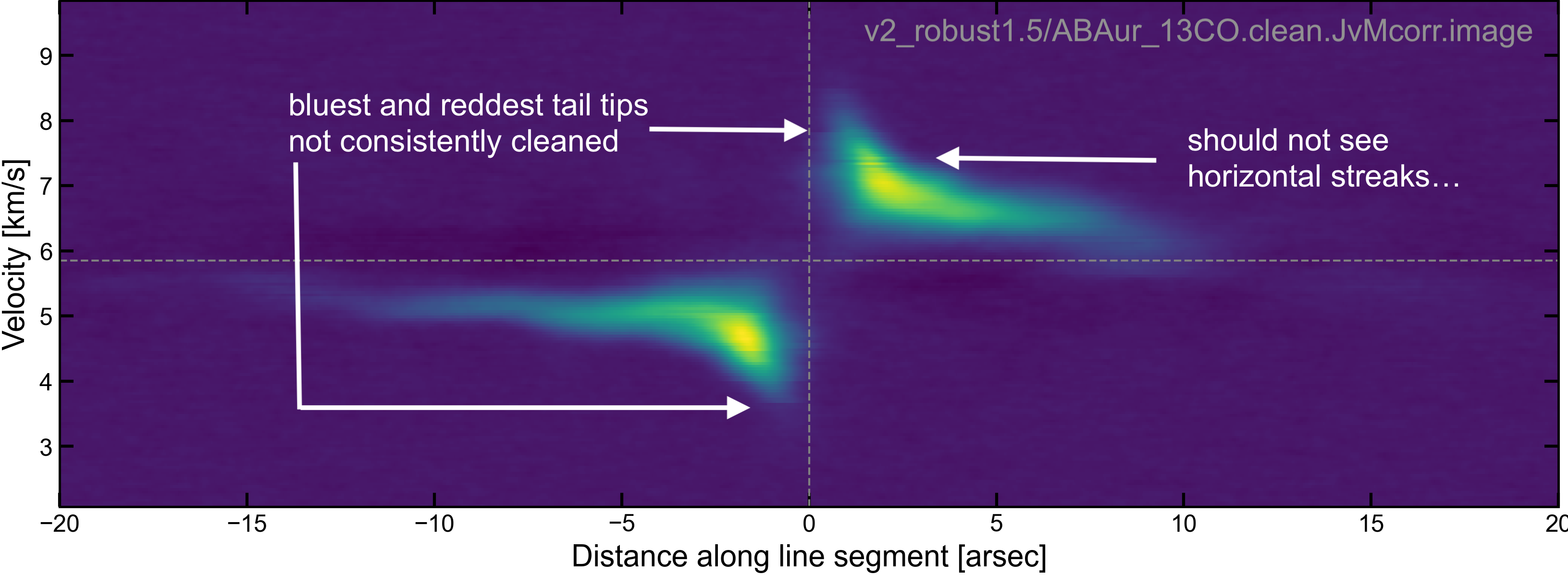
The tails of 12CO and 13CO emission at the bluest and reddest channels in the clean image stop abruptly, as if they have not been cleaned. [This can be seen in position-velocity maps below as a truncation of the tails in JvM-corrected images. The downscaled-by-epsilon residuals helps to make the problem really visually obvious.]
4th round of imaging experiments#
4th imaging approach taken: Masking emission with auto-multithresh and the Huang et al. (2021) parameters, but kickstarting auto-multithresh with a mask made from a model
Thinking back to one of Ryan’s ideas: “Take a dirty image, clean it a little bit, and define a mask by where the emission is over some threshold.” This seems like a good way that we could develop more precise masks.
Figuring out how to make a mask from a clean model
After plotting contours of some of the above cleaned images and imagining how well these contours would serve as an initial mask, I found myself thinking about how I could get a smoother mask. This is how I got the idea of using a clean model to define a threshold mask.
The order of operations now becomes:
Make a model. Do this by cleaning down to a threshold of 10x the rms measured in the dirty image in line-free channels (so, not deeply cleaned, to minimize the chances of capturing unreal emission). For this clean, use a primary beam mask (
usemask='pb'andpbmask=0.2) in all channels, and no auto-multithresh. Also, remove the smallest multiscale Gaussian so that the model is composed of[0.1, 0.3, 0.6, 1., 2. arcsec]Gaussians.Translate this model into a mask, using a threshold you determine by experimentation. Currently I’m using 10x the mean. For reference, model units are in Jy/pixel.
From here, it’s the same as before. Do one initial round of cleaning with the (model) mask, and without auto-multithresh. For this round set
niter=cycleniter=1(it’s important thatniter=cycleniter, and both=1simply so that the least amount of cleaning happens).Restart
tclean, now with auto-multithresh turned on, and givetcleaninstructions to pick up where the initial clean left off.
Translating a model image into a mask was somewhat non-trivial for me (I didn’t find the makemask and ia.calcmask tasks straightforward to use at first). Below is an example of how the model masks look, created from the model image by taking a cut at a threshold value of 10x the mean of the model pixel values.
There perhaps are some rogue white contour blobs (circles near the edge of the field of view) that should be removed. This would have to be done by hand, because increasing the cut threshold value (to e.g. 20x the mean) would shrink the mask so it no longer covers the diffuse emission, which would be defeating the whole point. But the other white contour blobs, within the realm of the disk, are seeds for auto-multithresh to pick up from. That’s the beauty of it: this mask doesn’t need to be perfect. Auto-multithresh will grow this mask how it needs to.
Imaging with auto-multithresh kickstarted with the mask from a clean model
As a first step, I used the exact masks generated above (i.e., I did no removing of any blobs by hand).
Below is an example of how the initial mask is grown over the course of the auto-multithresh cycles (in this case, C18O, 5 major cycles). The solid white regions represent the initial mask, and the white contours is the mask on the very last round:
Results: Cleaning is still discontinuous in velocity space, very few major cycles, negative bowling in central channels
Most troubling problem (most apparent at lower robust): The strange discontinuous cleaning in velocity space is still present (e.g. 7.362 km/s in 13CO). It is still the case with 12CO and 13CO that the number of autothresh iterations (i.e. major cycles) is only 1 or 2, which makes me think this could be the reason for the discontinous cleaning in velocity space.
The emission distribution in the background sky changes as a function of channel – it looks nice and even/random at the tail channels, and then quite patchy at the central channels. [Spoiler alert: It’s negative bowling due to missing short uv-spacings. See next page.]
Pause to reflect#
Let’s take stock of where we are after all these experiments. At this point, …
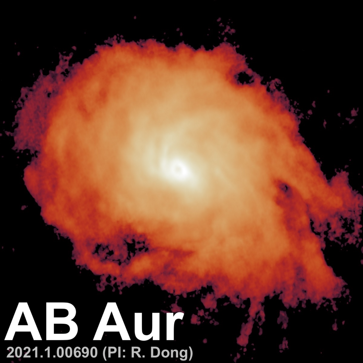
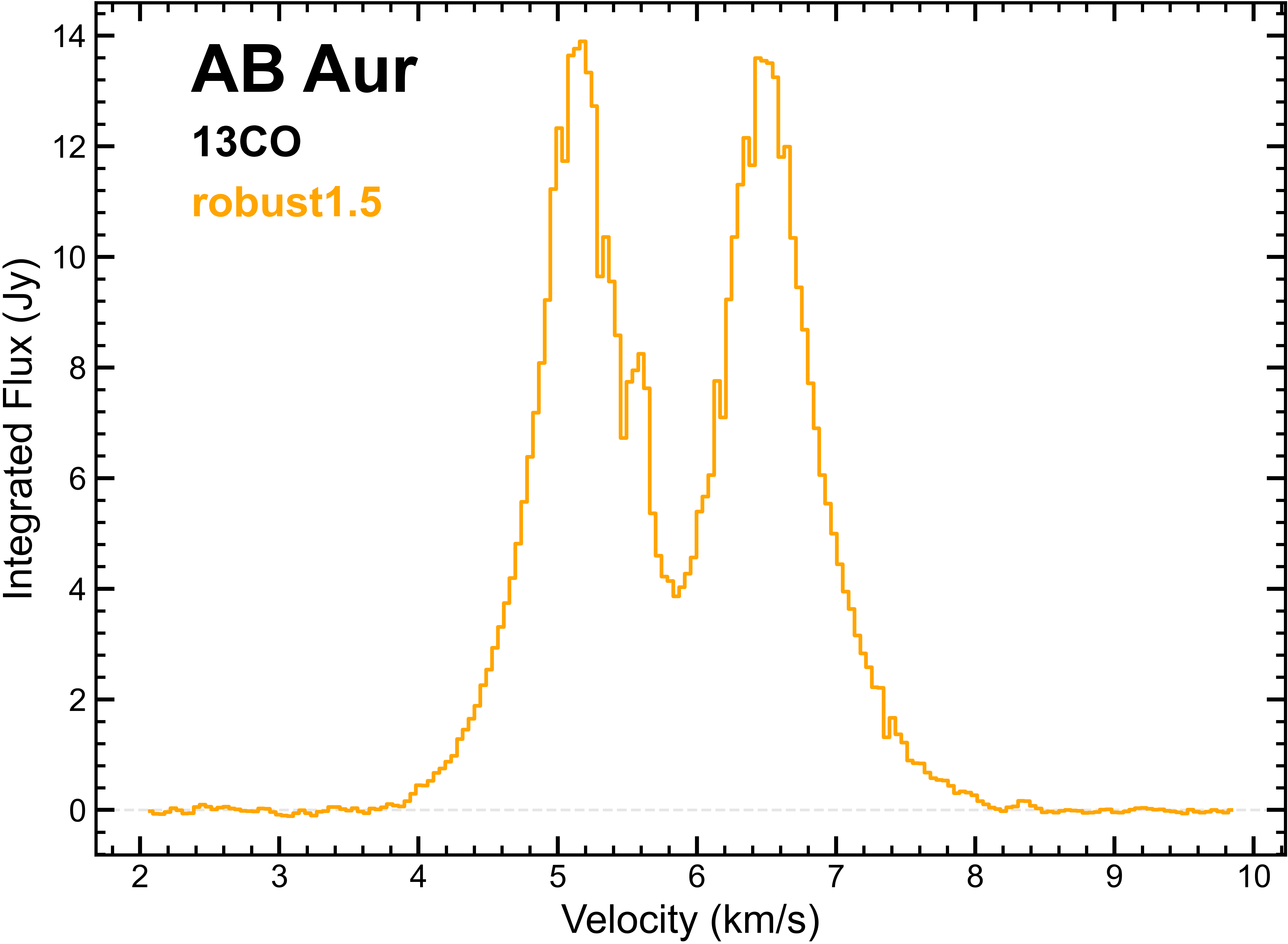
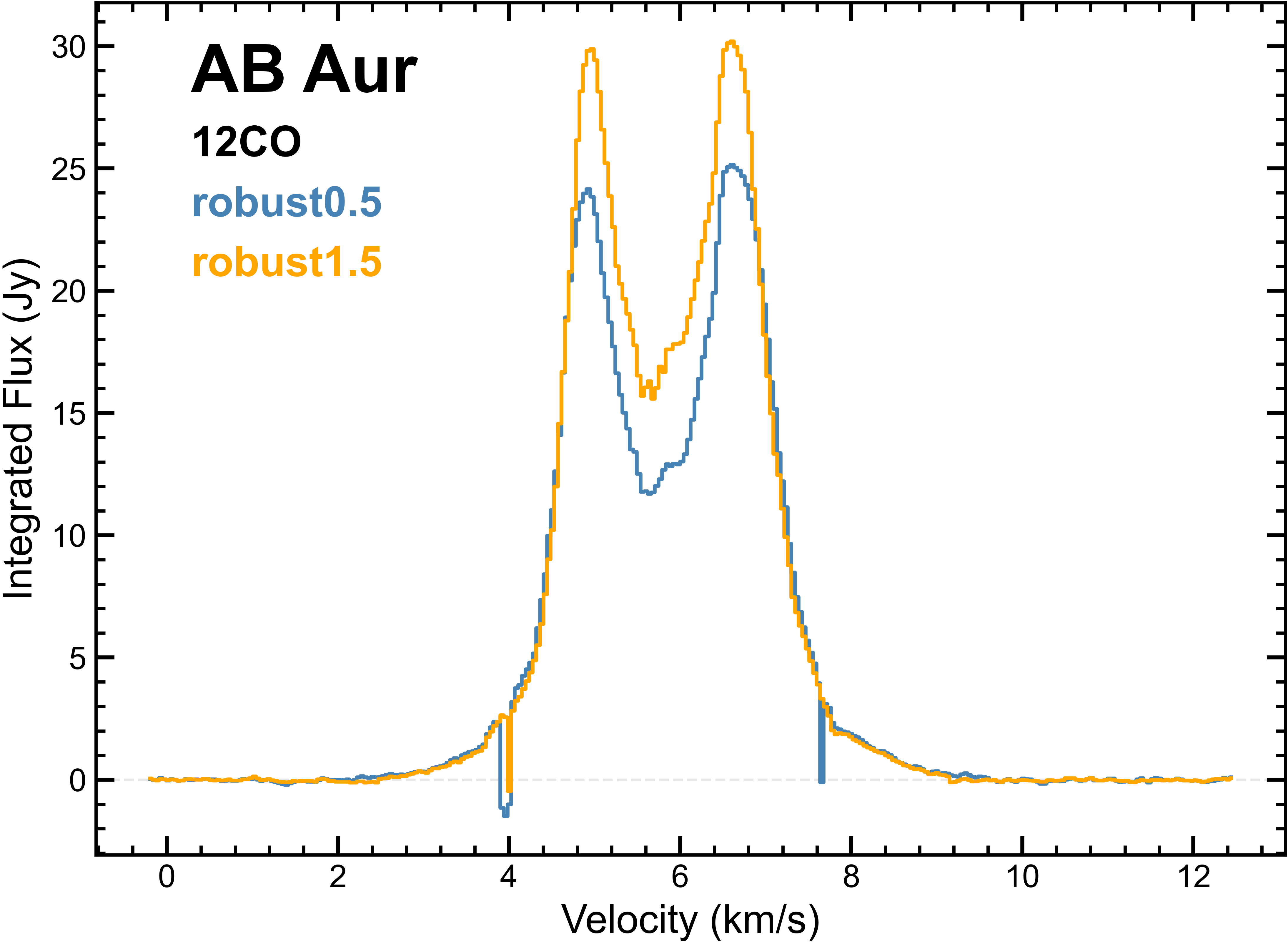
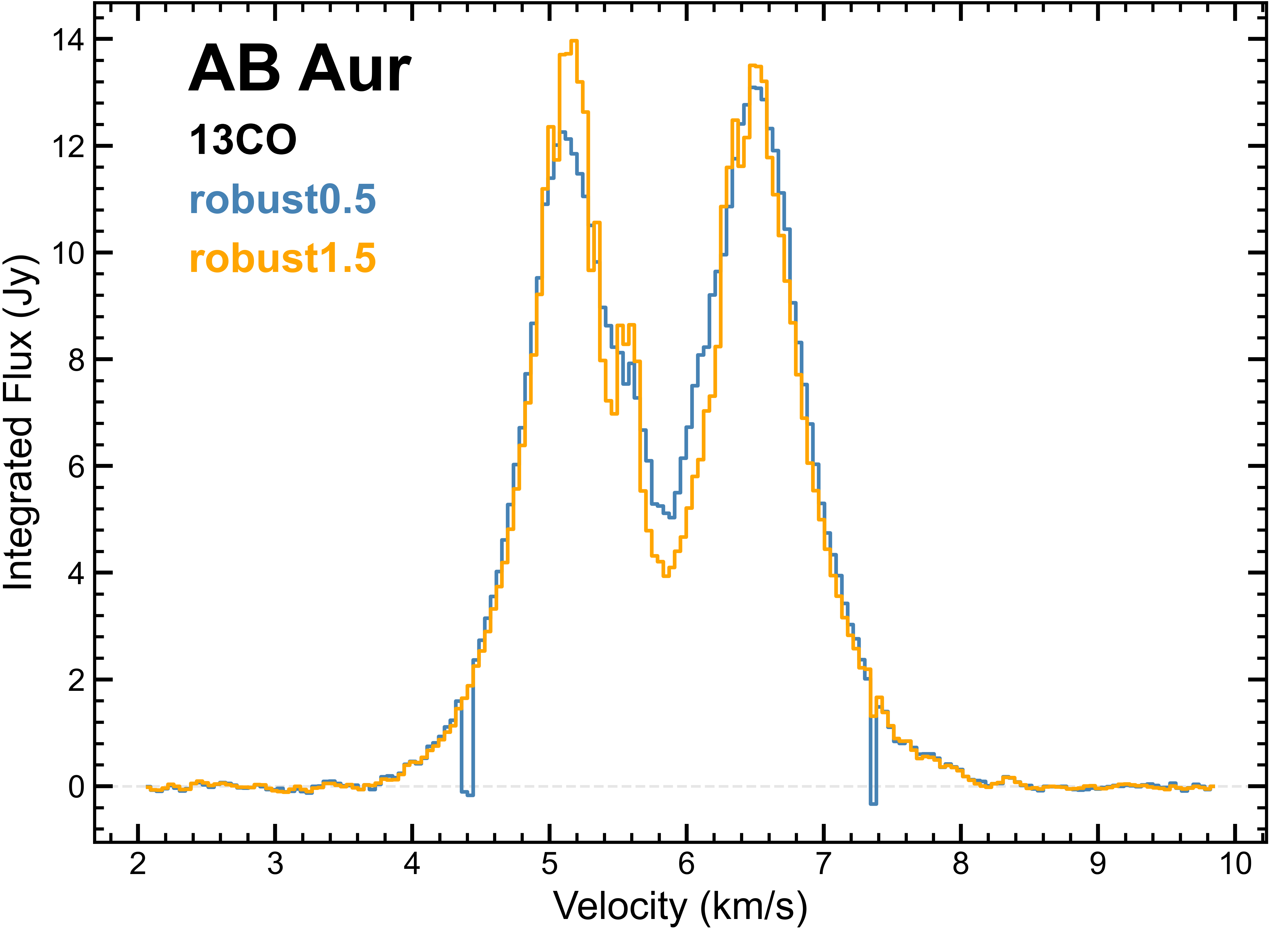
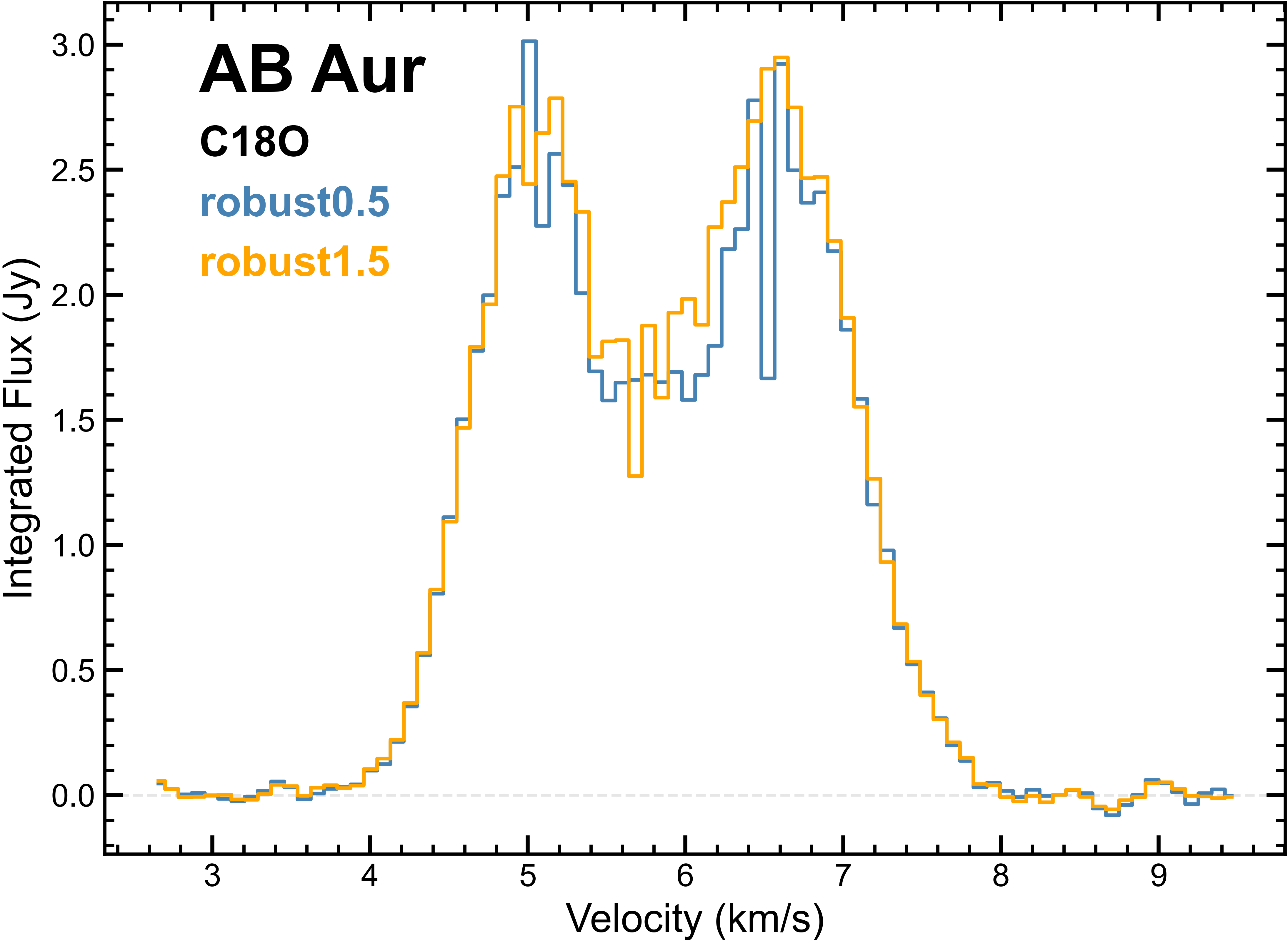
… the image cubes look like this:
… I discovered that, if I want to re-grid onto a chosen velocity grid, then I shouldn’t be working with measurement sets that have already had cvel2 applied (!).
I therefore went back to step 4 and undid the cvel2 step, such that all the measurement sets are in the TOPO frame.
… I reached out to the NAASC to arrange a virtual chat to get some input and new ideas.
I received written input from Amanda Kepley and met with Ryan Loomis – both were extremely helpful. The next page gives a summary of the new understanding I gained and motivation for the imaging strategy we consequently adopted for this program.