
Restoring the Pipeline Calibration#
This is also known as “Generating the calibrated visibilities”. (If you do a f2f visit to the NAASC, your data will be staged on NAASC computers and all of the following will be done for you before you even arrive!).
There are a couple different paths, depending on whether your program was calibrated by the pipeline or manually. See ALMA QA2 Data Products for Cycle 8, Section 5 (page 13), or this Knowledgebase article. Our program was calibrated by the pipeline, so we follow “Section 5.2: Running the scriptForPI.py in the case of pipeline-calibrated data”. Section 5.4 is also helpful: “Section 5.4: Saving disk space during and after the execution of the scriptForPI.py.”
Restoring the pipeline calibration using scriptForPI.py#
First, find the
scriptForPI.pyin the directory calledscript. Confirm that the file*pprequest.xmlis also present (it should be, it’s an indicator that the program was pipeline calibrated).
Understanding the directory substructure
Once downloaded and untarred, all data should fall into the standardized directory structure:
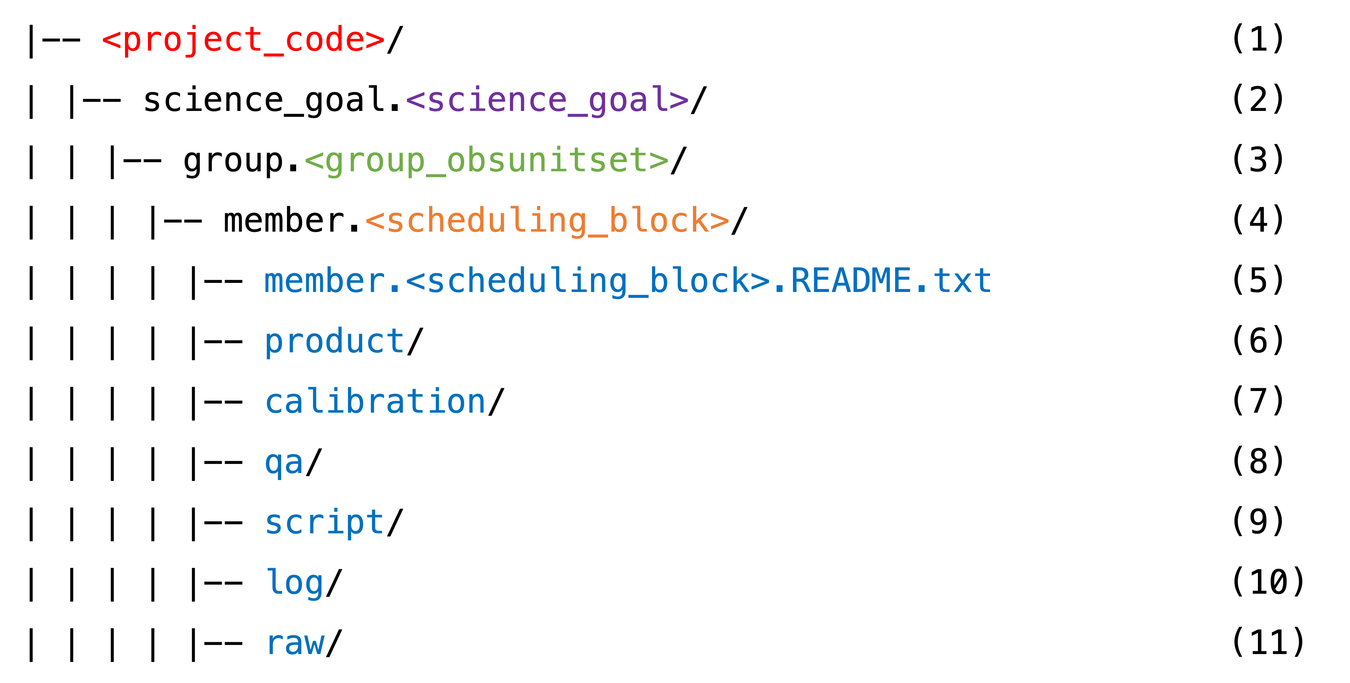
(1) The ALMA project code, or program ID. Ours is 2021.1.00690.S.
(2) The Science Goal ID. These are originally set up by the PI in the OT during proposal preparation. We have just one: uid___A001_X15a2_Xb69.
(3) The Group ObsUnitSet (a.k.a. GOUS). In our case there is just one: uid___A001_X15a2_Xb6a.
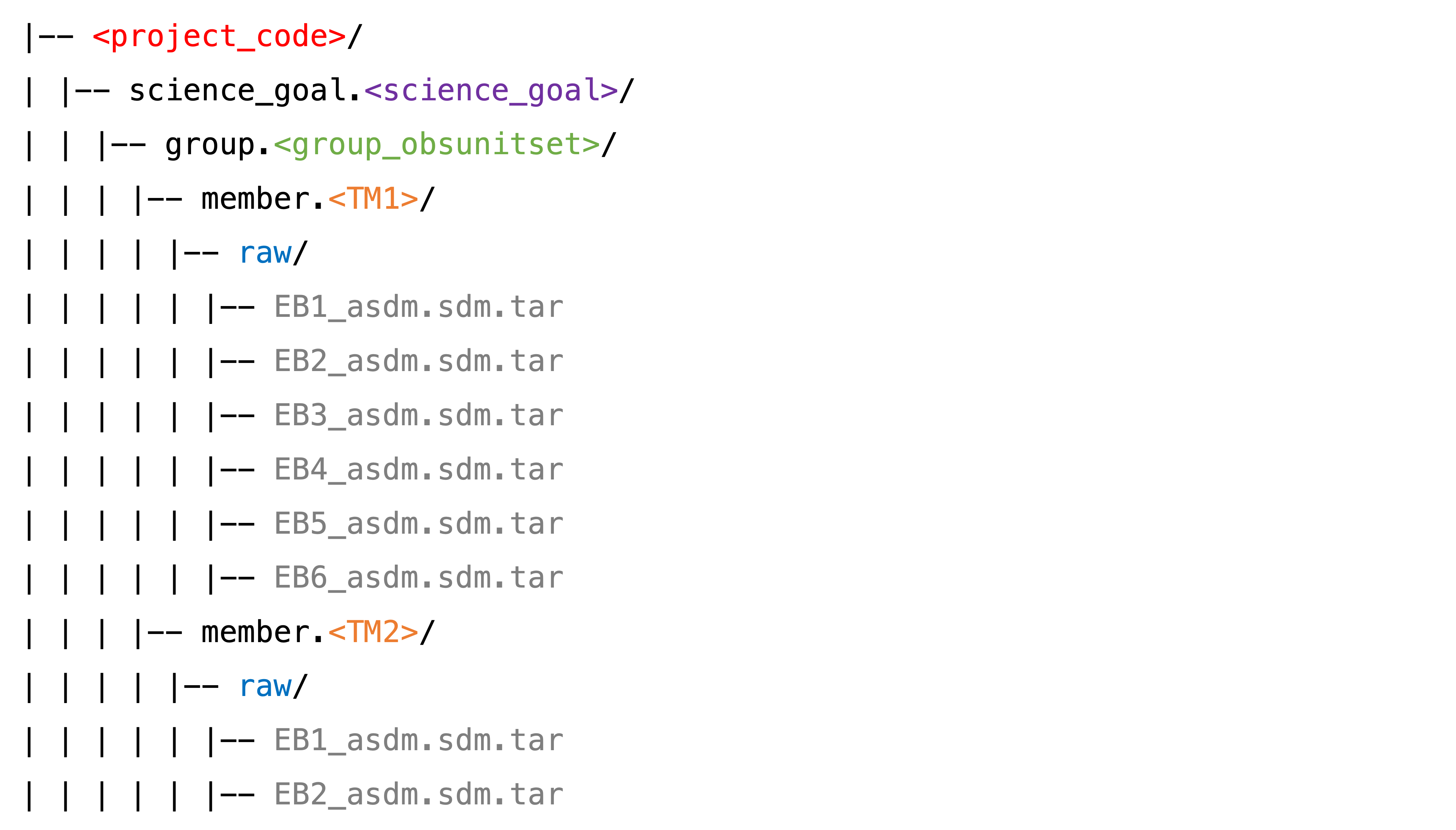
(4) The Member ObsUnitSet (a.k.a MOUS, a.k.a. Scheduling Block, a.k.a. SB). QA2 is carried out at this level. In our case, we have two (uid___A001_X15a2_Xb6b and uid___A001_X15a2_Xb6d) – one for each array configuration. The long-baseline configuration MOUS is also referred to as TM1, and the short-baseline configuration as TM2. The pipeline is run on each MOUS separately (and thus also delivered to the PI separately) – at least as of Cycle 8!
Each of our MOUSes contain multiple execution blocks (EBs). QA0 is carried out on the EB level. All of the following directories (6-11) contain all the files for each EB in each MOUS, where the file name starts with the EB ID. For example, our TM2 (short-baseline MOUS) directories contain all the files for EB1 uid___A002_Xf7ad58_Xd406 and for EB2 uid___A002_Xf8f6a9_X15c79.
(5) A very helpful file that explains the directory structure and file types.
(6) Contains the pipeline-generated image products (fits files).
(7) Contains the all-important calibration tables, and other things for restoring the pipeline calibration.
(8) Contains the blessing that is the Weblog. It also contains the Quality Assurance (QA) reports on the MOUS level (QA1) and the EB level (QA0).
(9) Contains the absolutely crucial scriptForPI.py – what you need to restore the pipeline calibration.
(10) Contains the CASA commands log from the QA2 processing.
(11) Contains the data! The raw visibilities in the native ALMA format (the ASDM). In our case:
More details can be found in ALMA QA2 Data Products for Cycle 8, Section 3 and 4.
It is important to restore the pipeline calibration using the same version of
CASAas the pipeline originally did. Check your weblog or QA reports to find out. Here we use version 6.2.1.7 (appropriate for Cycle 8).Open
CASAin thescriptdirectory, with the pipeline functions loaded:
~$ cd 2021.1.00690.S/science_goal.uid___A001_X15a2_Xb69/group.uid___A001_X15a2_Xb6a/member.uid___A001_X15a2_Xb6d/script
script$ casa --pipeline
Then, if you’re ready (this could take ~a day), execute
scriptForPI.py:
script$ execfile('member.uid___A001_X15a2_Xb6d.scriptForPI.py')
Or, if you’ve consulted Section 5.4: Saving disk space during and after the execution of the scriptForPI.py, set the selected flags and then execute scriptForPI.py:
script$ SPACESAVING=3
script$ execfile('member.uid___A001_X15a2_Xb6d.scriptForPI.py')
Upon completion, a new directory should have been created (in the member.<scheduling_block>/ level) called calibrated, which contains a measurement set, or MS file, for each execution block. For the TM2, or short-baselines, scheduling block where we have 2 execution blocks, the contents of the calibrated folder should look like this:
products -> ../calibration
rawdata
uid___A002_Xf7ad58_Xd406.ms -> working/uid___A002_Xf7ad58_Xd406.ms
uid___A002_Xf7ad58_Xd406.ms.flagversions -> working/uid___A002_Xf7ad58_Xd406.ms.flagversions
uid___A002_Xf8f6a9_X15c79.ms -> working/uid___A002_Xf8f6a9_X15c79.ms
uid___A002_Xf8f6a9_X15c79.ms.flagversions -> working/uid___A002_Xf8f6a9_X15c79.ms.flagversions
working
Repeat steps 3 and 4 for the other scheduling block,
member.uid___A001_X15a2_Xb6b. Upon completion, the newmember.uid___A001_X15a2_Xb6b/calibrateddirectory should contain 6 MSes, one for each execution block.
The uid*.ms measurement sets
These MS files contain all original spectral windows and both the calibrated and uncalibrated data. The calibrated data can be found in the MS table column 'CORRECTED_DATA'.
Splitting out the science spectral windows and target source#
The following may or may not have been done already by scriptForPI.py (you may need to set the DOSPLIT variable to DOSPLIT=True). Refer to Section 5.5: Splitting out the calibrated data at the end of running the scriptForPI.py.
Split out the science spectral windows. Here again we start with the short-baseline SB.
# In a CASA terminal and in the right directory: member.uid___A001_X15a2_Xb6d/calibrated/
import glob
vislist = glob.glob('*[!_t].ms')  # should be ['uid___A002_Xf7ad58_Xd406.ms', 'uid___A002_Xf8f6a9_X15c79.ms']
for myvis in vislist:
    msmd.open(myvis)
    targetspws = msmd.spwsforintent('OBSERVE_TARGET*')
    sciencespws = []
    for myspw in targetspws:
        if msmd.nchan(myspw)>4:
            sciencespws.append(myspw)
    sciencespws = ','.join(map(str,sciencespws))
    msmd.close()
    split(vis=myvis,outputvis=myvis+'.split.cal',spw=sciencespws)
This creates the uid*.ms.split.cal measurement sets.
The uid*.ms.split.cal measurement sets
These MS files contain contain the science target AND the calibrators, but only the science spectral windows.
Save the original flags.
# In a CASA terminal, in e.g., member.uid___A001_X15a2_Xb6d/calibrated/
import glob
vislist=glob.glob('*.ms.split.cal')
for vis in vislist:
    flagmanager(vis=vis,
                mode='save',
                versionname='original_flags')
Split off the science target, and save those flags too.
# In a CASA terminal, in e.g., member.uid___A001_X15a2_Xb6d/calibrated/
for vis in vislist:
    outputvis = vis+'.source'
    split(vis=vis,
      intent='*TARGET*', # split off the target sources by intent
      outputvis=outputvis,
      datacolumn='data')
    os.system('rm -rf ' + outputvis + '.flagversions')
    flagmanager(vis=outputvis,
                mode='save',
                versionname='original_flags')
This creates the uid*.ms.split.cal.source measurement sets.
The uid*.ms.split.cal.source measurement sets
These MS files contain contain only the science target, and only the science spectral windows. The calibrated data should be in the MS table column 'DATA'.
For the TM2, or short-baselines, scheduling block where we have 2 execution blocks, the contents of the calibrated folder should now look like this:
products -> ../calibration
rawdata
uid___A002_Xf7ad58_Xd406.ms -> working/uid___A002_Xf7ad58_Xd406.ms
uid___A002_Xf7ad58_Xd406.ms.flagversions -> working/uid___A002_Xf7ad58_Xd406.ms.flagversions
uid___A002_Xf7ad58_Xd406.ms.split.cal.flagversions
uid___A002_Xf7ad58_Xd406.ms.split.cal.source
uid___A002_Xf7ad58_Xd406.ms.split.cal.source.flagversions
uid___A002_Xf8f6a9_X15c79.ms -> working/uid___A002_Xf8f6a9_X15c79.ms
uid___A002_Xf8f6a9_X15c79.ms.flagversions -> working/uid___A002_Xf8f6a9_X15c79.ms.flagversions
uid___A002_Xf8f6a9_X15c79.ms.split.cal.flagversions
uid___A002_Xf8f6a9_X15c79.ms.split.cal.source
uid___A002_Xf8f6a9_X15c79.ms.split.cal.source.flagversions
working
Repeat steps 1-3 for the long-baselines scheduling block,
member.uid___A001_X15a2_Xb6b.
In summary, we start step 1 with 8 separate measurement sets (i.e., 8 of uid*.ms.split.cal.source) which contain only the science spectral windows for only the science target.