
Scripts for Step 4 - Prepare the lines:
step4_prepare_lines.py # main script
step4_detour.py # for phase alignment
dictionary_data.py # loads data_dict
step1_utils.py # loads multiple functions
analysisUtils (analysis_scripts/) # for channel strings
Apply Self-Calibration Solutions#
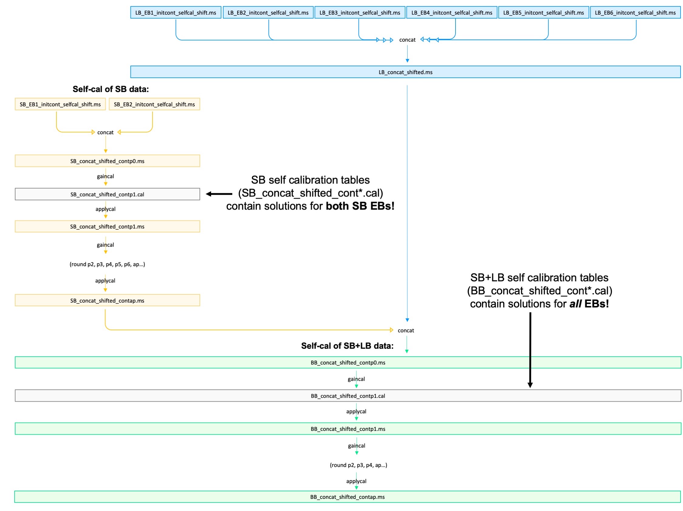
At this point, we have eight phase-aligned EBs (6 LBs and 2 SBs) with suffix _initlines_shift.ms, containing our line data. Each EB has the four line spectral windows (SPW 1-4). The averaged-down continuum spectral window (SPW 0) is also still tagging along for the ride.
We now wish to apply the calibration solutions that we generated from the continuum self-calibration in Step 3. The calibration solutions are in calibration tables. Each one contains information that the others do not, so we need to apply them all, and in the same succession as they were generated.
Calibration tables generated using short-baseline data only |
Calibration tables generated using concatenated short-baseline + long-baseline data |
|---|---|
SB_contp1.cal |
BB_contp1.cal |
SB_contp2.cal |
BB_contp2.cal |
SB_contp3.cal |
BB_contp3.cal |
SB_contp4.cal |
BB_contp4.cal |
SB_contp5.cal |
BB_contap.cal |
SB_contp6.cal |
|
SB_contap.cal |
It would be most intuitive to concatenate the SB line data (i.e., concatenate the two short baseline _initlines_shift.ms measurement sets), and then apply each of the calibration tables in the left column above (SB_contp1.cal, then SB_contp2.cal, and so on) – and then concatenate that resulting SB data with the LB data (i.e., the six long baseline _initlines_shift.ms measurement sets), and apply the self calibration tables in the right column above (BB_contp1.cal, then BB_contp2.cal, and so on) to that single giant measurement set. However, concatenating would use a lot of disk space (each MS is ~50 GB), and it would take applycal a lot of time to apply the solutions. As such, we keep the data in their separate execution blocks, and then at the very end, split out each spectral window and combine the corresponding spectral windows across executions.
Doing it this way, we face one complication: We generated our self calibration tables using concatenated data. This means that each calibration table is big, and contains solutions for multiple EBs. We need to apply each calibration table to only a subset of the data it was generated with. Below is a visual representation of the situation.
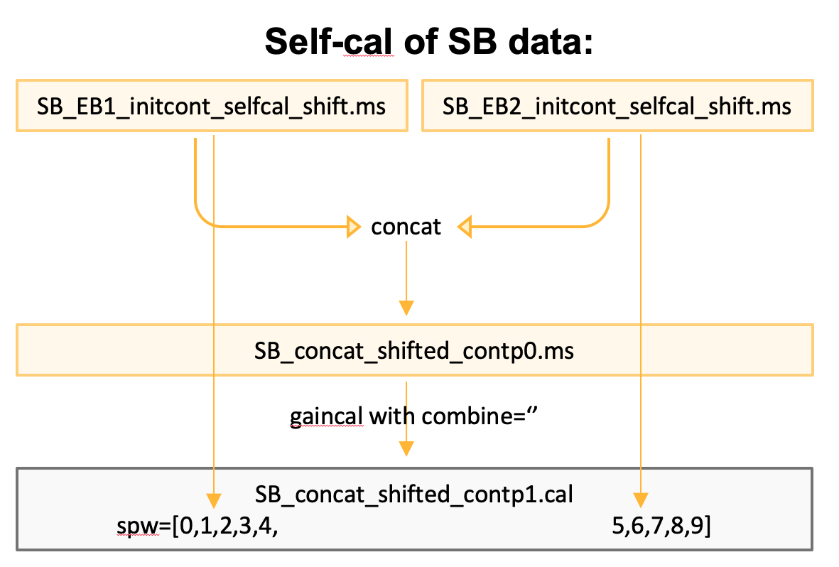
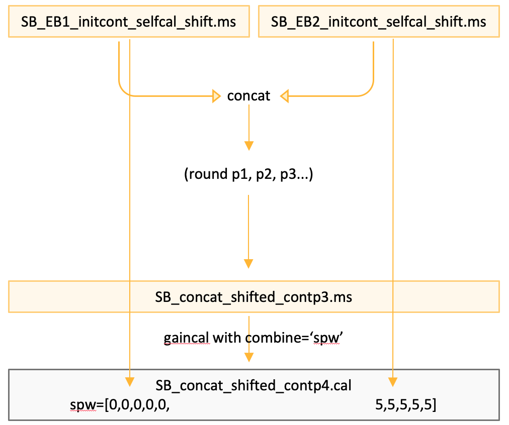
The applycal task spwmap parameter lets us take only a subset of the spectral windows contained within a calibration table, and apply those to the input MS. The trick is knowing how the mapping will work, because it requires accounting for the rounds where the combine='spw' parameter was or wasn’t set during gaincal. For example, compare these two SB calibration tables:
The same idea applies for the BB (SB+LB) calibration tables. Here is the same information but presented a different way:
SB_contp1.cal was gained on SB1 and SB2 with combine='', so it contains spws [0,1,2,3,4,5,6,7,8,9]
If we want to apply it to SB 1 (lines) only, we need spwmap=[0,1,2,3,4]
                   and to SB 2 (lines) only, we need spwmap=[5,6,7,8,9]

SB_contp3.cal was gained on SB1 and SB2 with combine='spw', so it contains spws [0,0,0,0,0,5,5,5,5,5]
If we want to apply it to SB 1 (lines) only, we need spwmap=[0,0,0,0,0]
                   and to SB 2 (lines) only, we need spwmap=[5,5,5,5,5]
The applycal task has another very useful parameter, gaintable, which we use to apply multiple calibration solutions in one call, but still in succession.
So with all that in mind, these are the required lists and combinations:

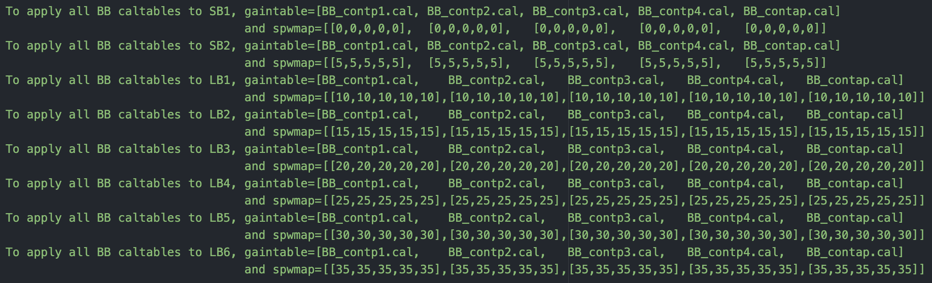
We do two “runs” of applycal; the first to apply the SB calibration tables, and the second to apply the SB+LB calibration tables. These are done separately (we do not feed in an uber gaintable and spwmap list) so that the applymode parameter can be set differently in the two cases. In the former, applymode='calflag' (calibrate and flag), and in the latter, applymode = 'calonly' (calibrate only).