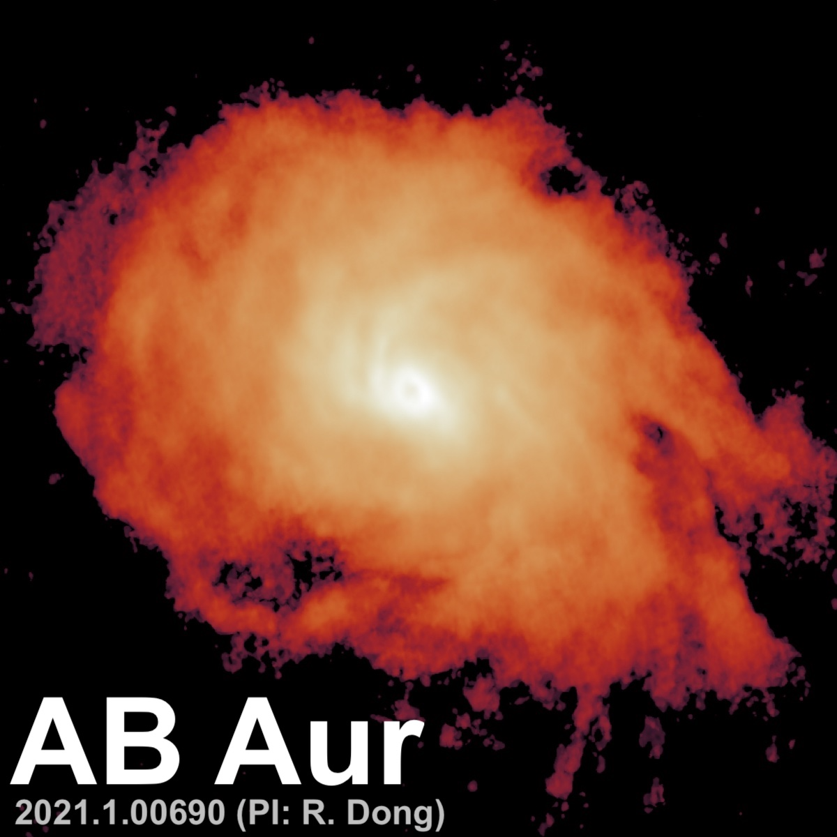
Step 1 Overview & Scripts#
In this step, we begin our post-processing of the continuum.
Scripts for Step 1 - Prepare the continuum:
step1_prepare_continuum.py # main script
dictionary_data.py # loads data_dict
step1_utils.py # loads multiple functions
selfcal_utils.py # necessary for an initial round of selfcal at the end
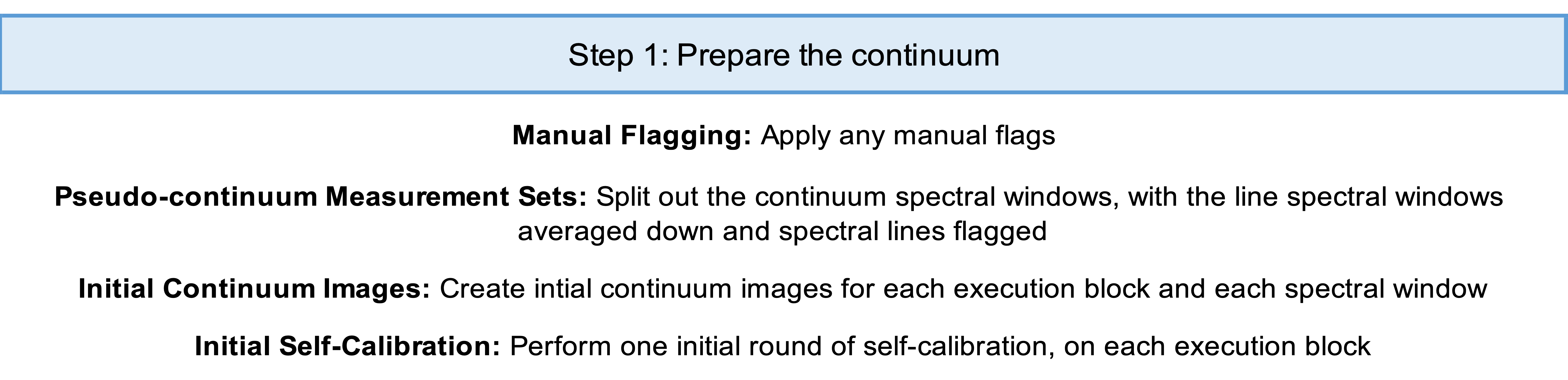
Manual Flagging: Before starting to work with the data, we should identify data we want to flag out, if any errors were identified during inspection of the weblog.
Pseudo-continuum Measurement Sets: We create pseudo-continuum datasets by flagging the line emission in each line SPW and spectrally averaging. We use the DSHARP function get_flagchannels to find the channels containing line emission in each SPW. In order to maximize the retained bandwidth (and achieve high SNR for per-SPW self calibration at a later step), we flagged channels \(\pm 6\) km/s from the \(^{13}\)CO \(J=2-1\) line center, and \(\pm 4\) km/s from the C\(^{18}\)O \(J=2-1\) line center. While these velocity ranges are narrower than the \(\pm 15\) km/s and \(\pm 25\) km/s velocity ranges flagged by MAPS and DSHARP, respectively, we confirmed that they capture all tail emission with a buffer of \(\geq1\) km/s by imaging the cubes and visually inspecting the channels. The continuum SPWs were spectrally averaged into 250 MHz channels (8 bins), whereas the line SPWs were averaged into a single 58.594 MHz channel (equal to the SPW bandwidth).
Initial Continuum Images: We create some initial images of the continuum data. We image each execution block, and spectral window, individually.
Initial Self-Calibration: To prepare each dataset for phase alignment, we performed an initial single round of phase self-calibration on each EB separately. We obtained the initial model by imaging each EB shallowly and interactively with Hogdom deconvolution (\(\delta\)-function clean components; Hogbom 1974). This initial round of self calibration increased the SNR in all EBs and visually improved the images.