Pseudo-continuum Measurement Sets

Pseudo-continuum Measurement Sets#

Flagging channels with line emission#

We want to remove our spectral lines to create a continuum-only measurement set. To do that, we have to take into account Doppler shifting of the lines (in the TOPO frame) over the course of the year. The six TM1 execution blocks were observed between 2022-07-17 and 2022-07-22; the two TM2 execution blocks were observed on 2022-04-19 and 2022-05-15.

I used the DSHARP function get_flagchannels (reductions_utils.py) to identify which channels to flag in each spectral window, given the rest frequency of the spectral line, and a choice of velocity range.

Relevant lines in step1_prepare_continuum.py

flagchannels_string = get_flagchannels(ms_file          = inputvis,
                                       ms_dict          = data_dict[EB],
                                       velocity_range   = data_dict[EB]['velocity_ranges'])
print('\nFor '+EB+', flagchannels_string = ', flagchannels_string)

Relevant lines in dictionary_data.py

velocity_ranges = np.array([np.array([ddisk.disk_dict['v_sys']-3., ddisk.disk_dict['v_sys']+3.]),
                            np.array([ddisk.disk_dict['v_sys']-4., ddisk.disk_dict['v_sys']+4.]),
                            np.array([ddisk.disk_dict['v_sys']-6., ddisk.disk_dict['v_sys']+6.]),
                            np.array([ddisk.disk_dict['v_sys']-10., ddisk.disk_dict['v_sys']+10.])])

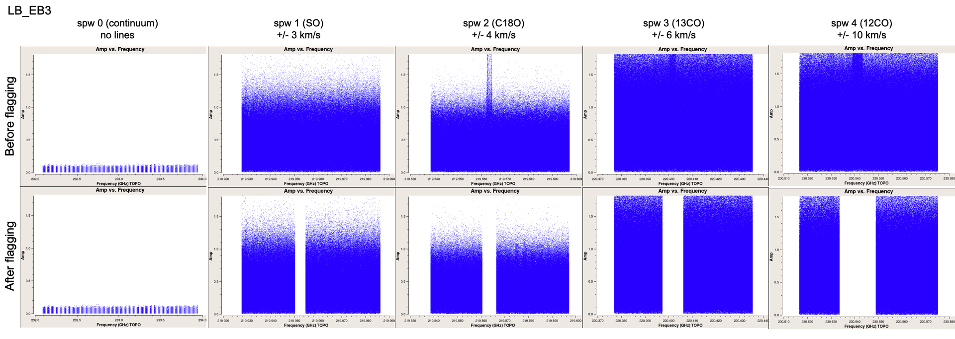
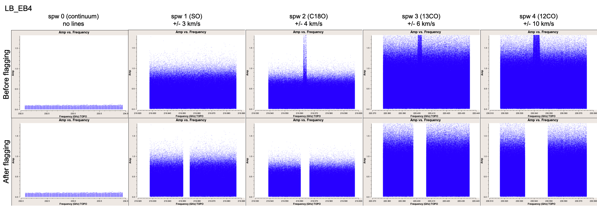
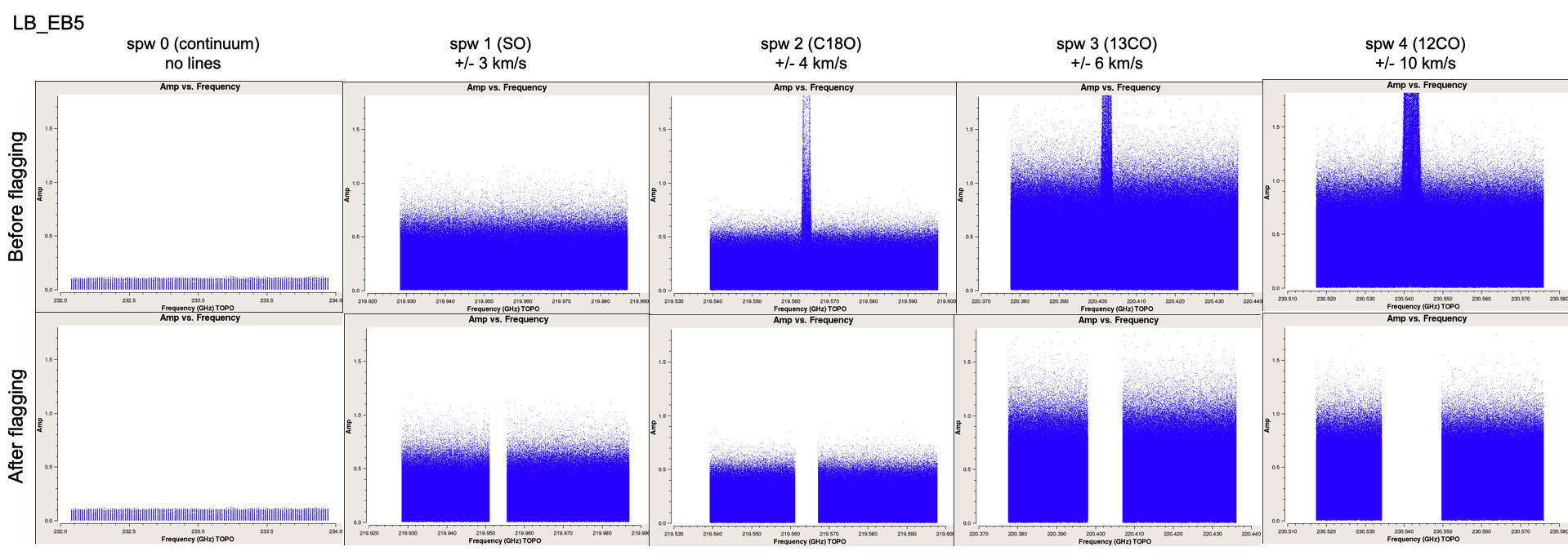
In order to maximize the retained bandwidth (and achieve high SNR for per-SPW self calibration at a later step), we flagged channels in wider or narrower ranges depending on the targeted spectral line (e.g. \(\pm 10\) km/s from the \(^{12}\)CO \(J=2-1\) line center, and \(\pm 6\) km/s from the \(^{13}\)CO \(J=2-1\) line center). Note that our velocity ranges are narrower than the velocity ranges flagged by MAPS and DSHARP. We confirmed that they capture all tail emission with a buffer of \(\geq1\) km/s by imaging the cubes and visually inspecting the channels.

Spectral averaging#

We average the continuum SPWs into 250 MHz channels (8 bins), whereas the line SPWs we average into a single 58.594 MHz channel (equal to the SPW bandwidth).

Relevant lines in step1_prepare_continuum.py

avg_cont(msfile         = inputvis,
         outputvis      = outputvis,
         flagchannels   = flagchannels_string,
         contspws       = data_dict[EB]['cont_spws'],
         width_array    = data_dict[EB]['width_array'],
         datacolumn     = 'data',
         field          = 'AB_Aur')

Relevant lines in dictionary_data.py

width_array = [8, 960, 960, 1920, 1920] # number of channels to average together

Visuals/results#

SB EB1#

Short-baseline execution block 1 (“SB EB1” or “SB1”), 19 April 2022. The top row shows our five SPWs in the context of the full frequency range of ALMA Band 6. The bottom row zooms into each SPW. The sky and rest frequencies of each target spectral line are overlaid. These bottom panels change as each EB is observed at a different time of year. Vertical lines are plotted in these panels for each channel they contain (only clear to see in the case of the continuum SPW with 128 channels).

Short-baseline execution block 1 (“SB EB1” or “SB1”), 19 April 2022. Visibility amplitude as a function of frequency, before and after flagging the lines in SPWs 1-4. The continuum spectral window (spw 0) is unchanged.

In hindsight…

Plots like these (with plotms) can be a lot clearer with avgtime='1e8', avgscan=True and avgbaseline=True.

SB EB2#

Short-baseline execution block 2 (“SB2”), 15 May 2022.

Short-baseline execution block 2 (“SB2”), 15 May 2022.

LB EB1#

Long-baseline execution block 1 (“LB1”), 17 July 2022.

Long-baseline execution block 1 (“LB1”), 17 July 2022.

LB EB2#

Long-baseline execution block 2 (“LB2”), 19 July 2022.

Long-baseline execution block 2 (“LB2”), 19 July 2022.

LB EB3#

Long-baseline execution block 3 (“LB3”), 20 July 2022.

Long-baseline execution block 3 (“LB3”), 20 July 2022.

LB EB4#

Long-baseline execution block 4 (“LB4”), 21 July 2022.