Scripts for Step 1 - Prepare the continuum:
step1_prepare_continuum.py # main script
dictionary_data.py # loads data_dict
step1_utils.py # loads multiple functions
selfcal_utils.py # necessary for an initial round of selfcal at the end
Initial Continuum Images#
Here we perform initial imaging of the continuum data. For each execution block, we image the aggregate continuum as well as each spectral window individually. With 8 execution blocks, each with 1 continuum SPW, 4 pseudo-continuum SPWs, and the combined-SPW aggregate, that’s 48 images in total.
Out motivation for doing this initial imaging is:
To check that the channel- and time-averaging didn’t do anything noticeably problematic to the data.
To get a sense of which execution blocks, and which spectral windows, are weak and which are strong (i.e. which have largest visible phase errors, which have largest SNR, etc). This will be useful for informing which EB to choose as a reference for phase alignment. We will (if possible) want to do (at least) one per-spw round of self-calibration, which will only be successful if we have high SNR in every spectral window.
To get familiar with the current state of the data, so we can later gauge how much or little improvement we see after phase alignment (Step 2) and self-calibration (Step 3).
I used the DSHARP function image_each_obs (reductions_utils.py) which loops through all the observations in a measurement set and images them individually, as well as makes images for each spectral window alone. Not wanting to clean 48 images interactively, I used the clean threshold values found by the pipeline (the hif_makeimages (mfs) task in the weblog). The values are set in dictionary_data.py; note that the threshold is the same or similar for the SPW 0 (continuum SPW) image as for the aggregate continuum image.
image_each_obs(ms_dict      = data_dict[EB],
               inputvis     = data_dict['NRAO_path']+data_dict[EB]['_initcont.ms'],
               mask         = SB_mask,
               scales       = SB_scales,
               imsize       = SB_imsize,
               cellsize     = SB_cellsize,
               contspws     = data_dict[EB]['cont_spws'],
               # threshold    = '0.0mJy', # this is taken care of inside image_each_obs() through ms_dict
               interactive  = False)
SB_pipeline_cont_cleanthresh           = 0.18, #mJy; from weblog hif_makeimages (aggregate)
SB_pipeline_cont_cleanthresh_perspw    = [0.18, 0.66, 0.57, 0.78, 0.7], #mJy; from weblog hif_makeimages (mfs)
LB_pipeline_cont_cleanthresh           = 0.060, #mJy; from weblog hif_makeimages (aggregate)
LB_pipeline_cont_cleanthresh_perspw    = [0.062, 0.26, 0.25, 0.2, 0.11], #mJy; from weblog hif_makeimages (mfs)
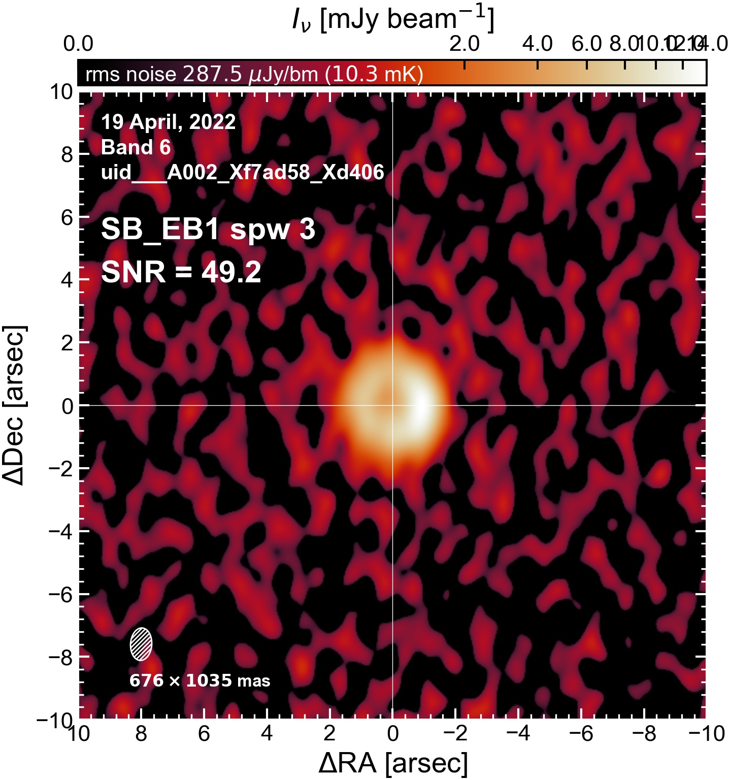
The following are the resulting images of the continuum for each execution block.
SB EB1#


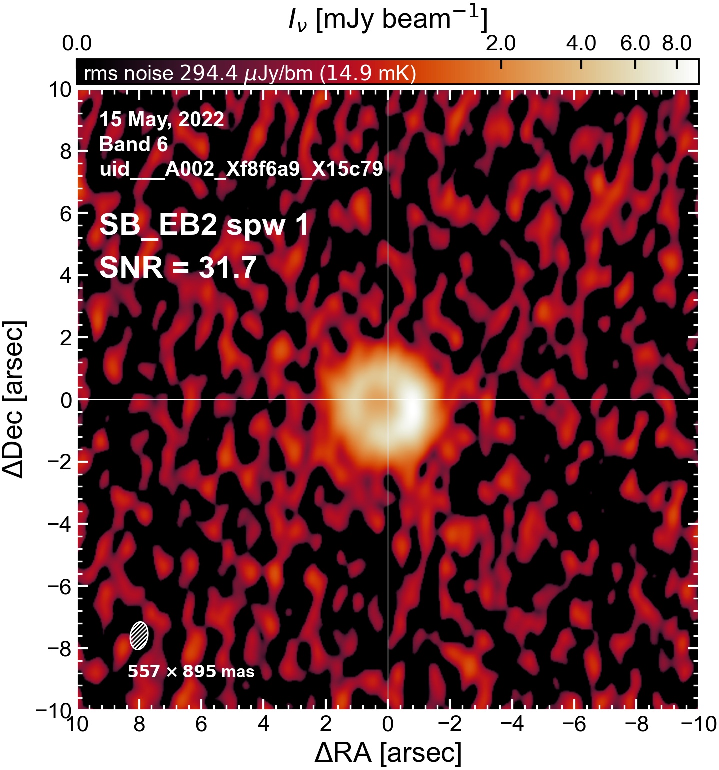
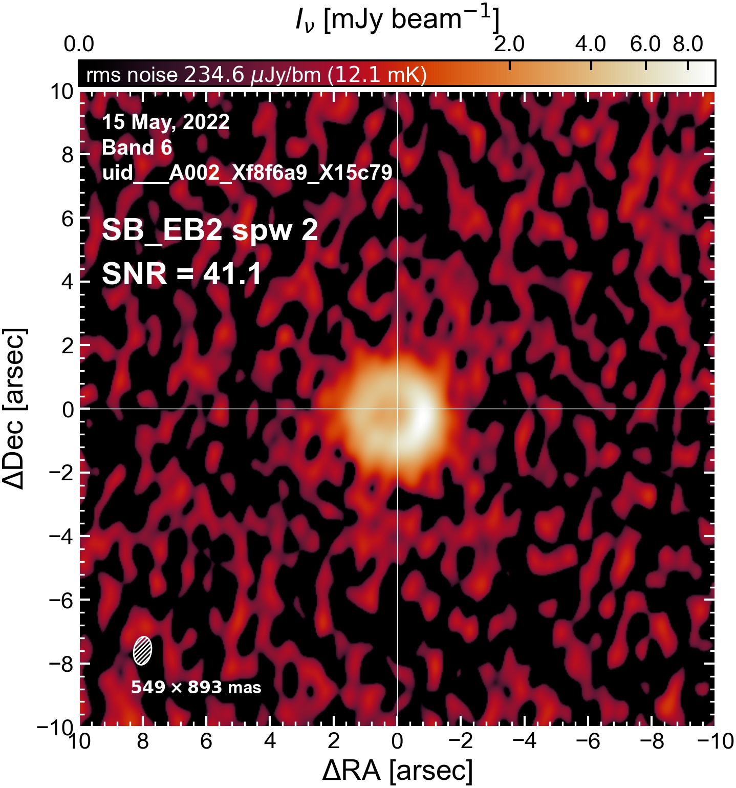
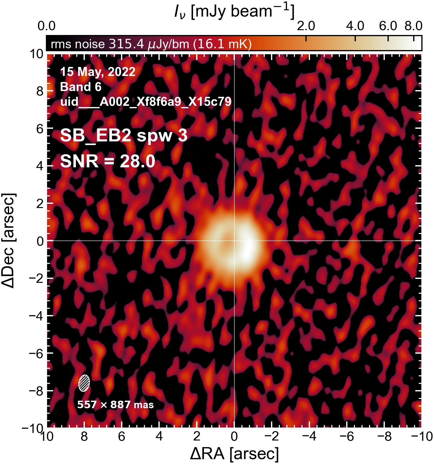
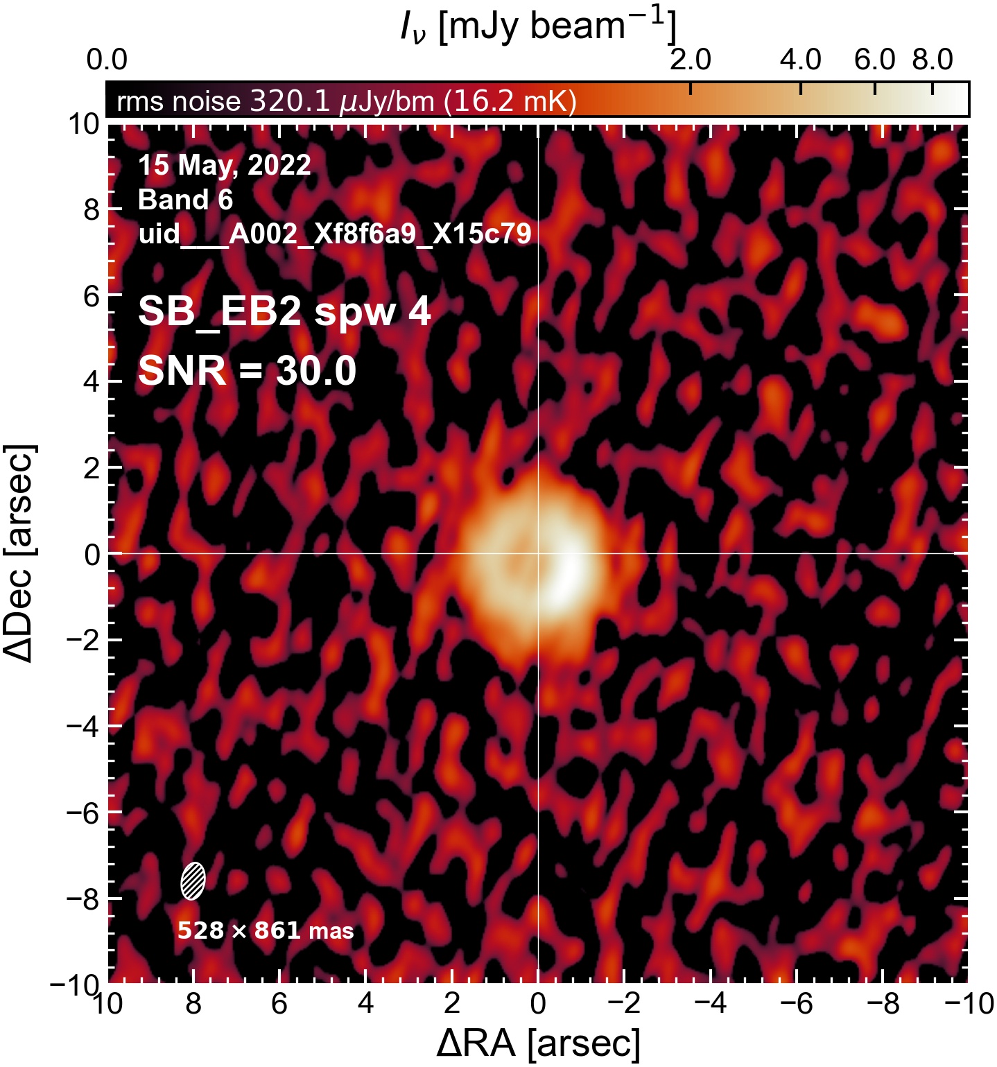
SB EB2#


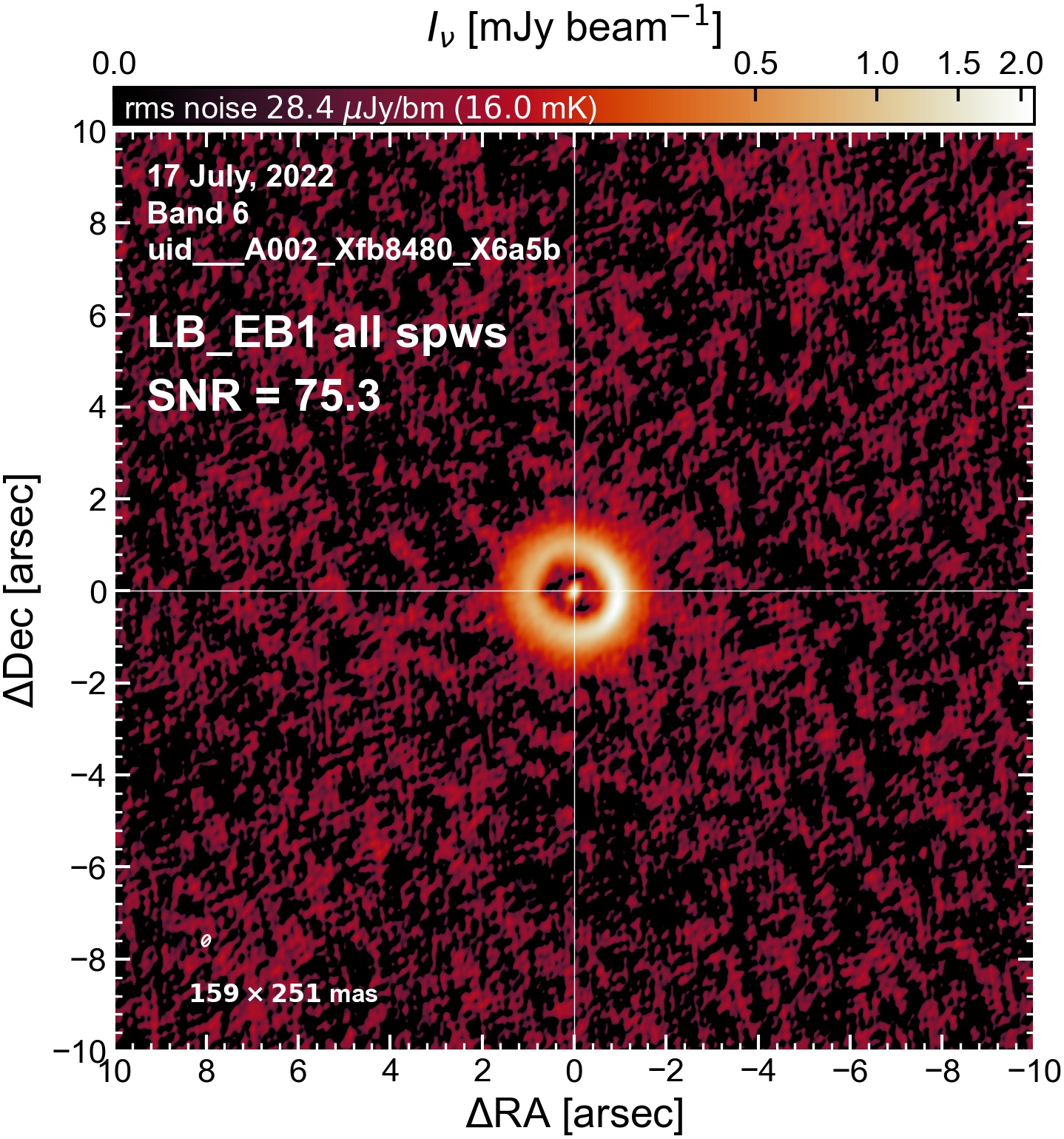
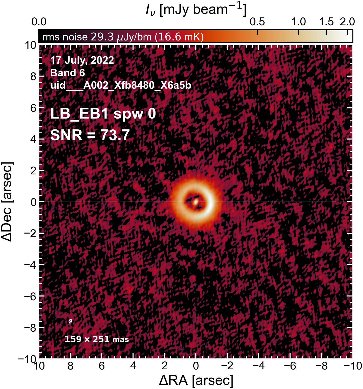
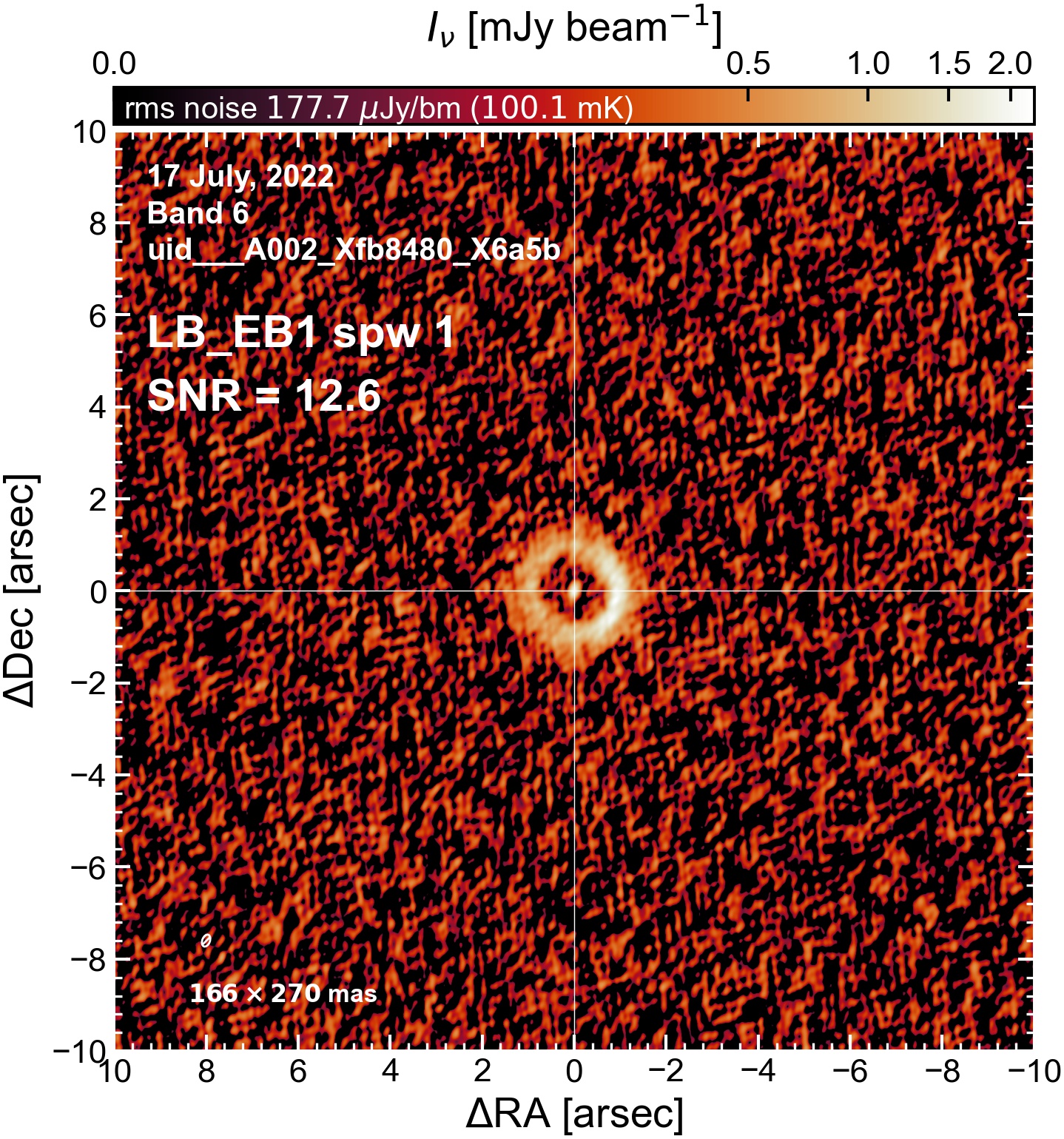
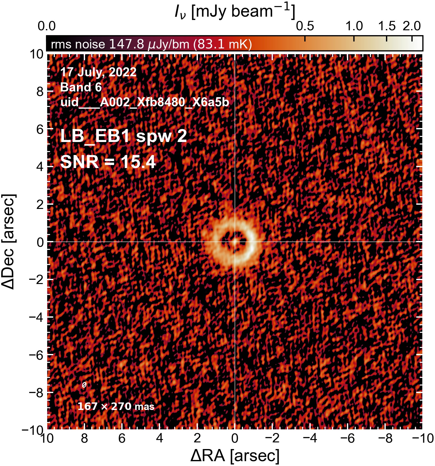
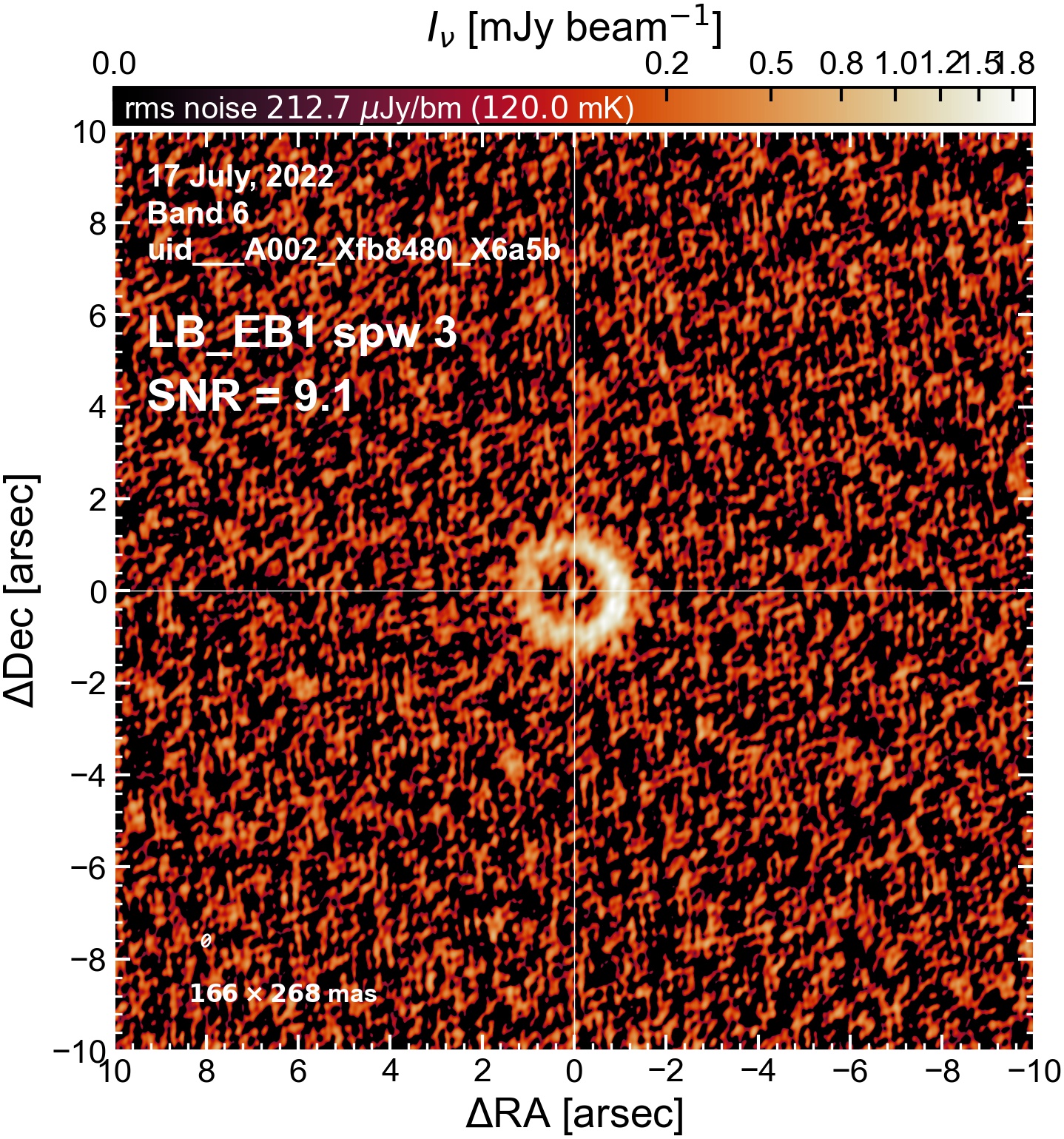
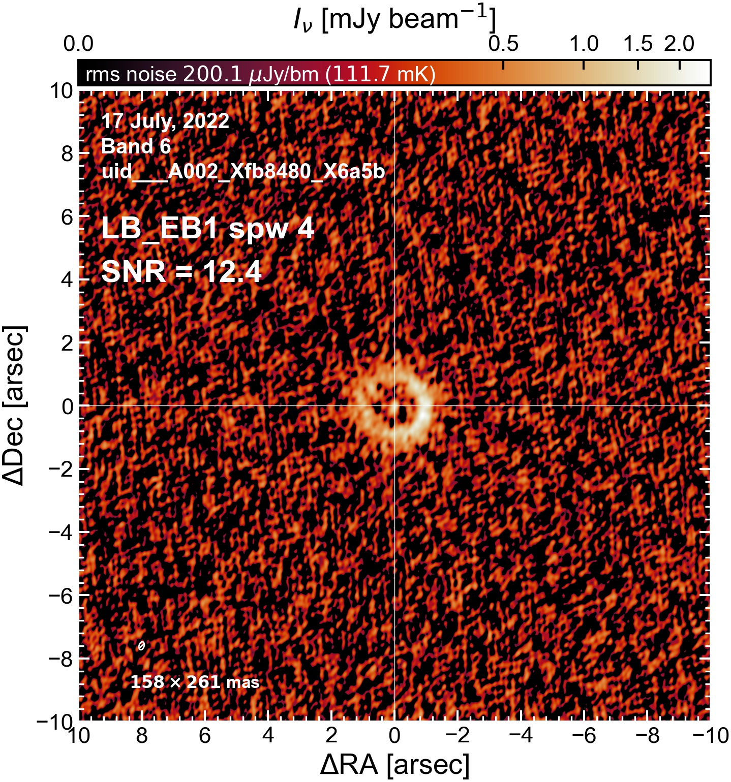
LB EB1#
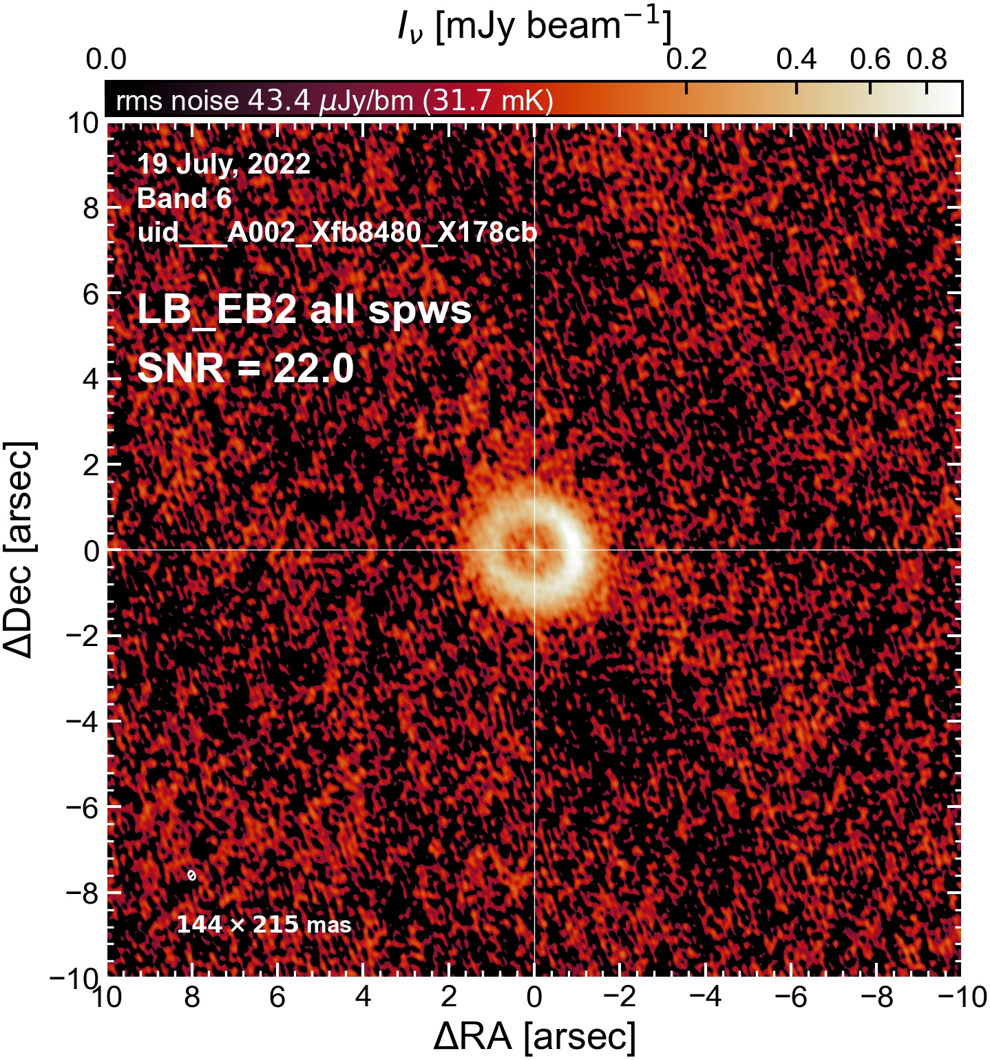
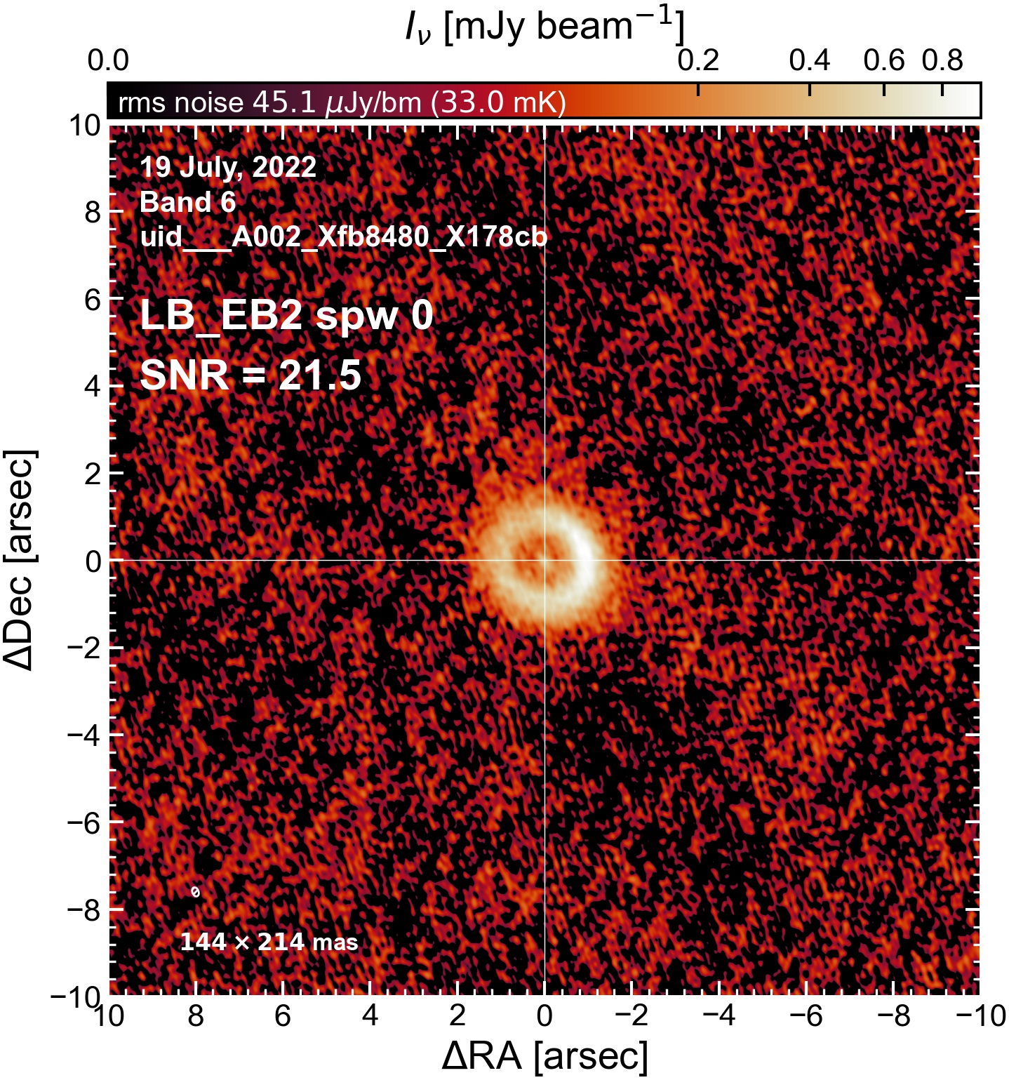
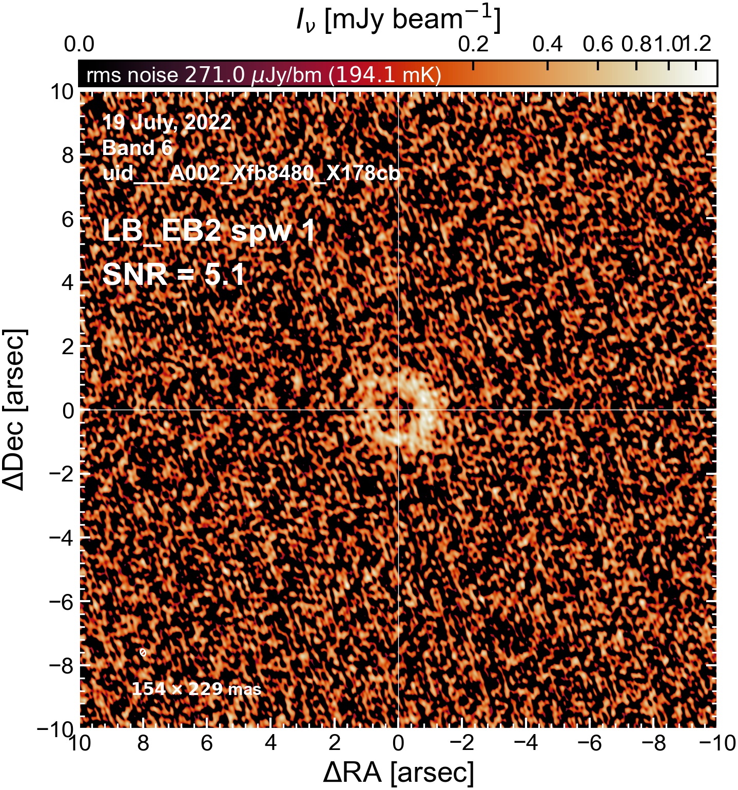
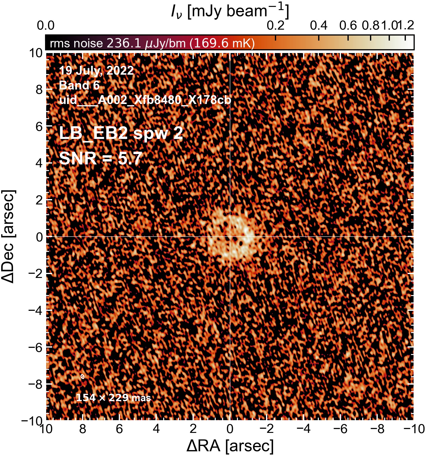
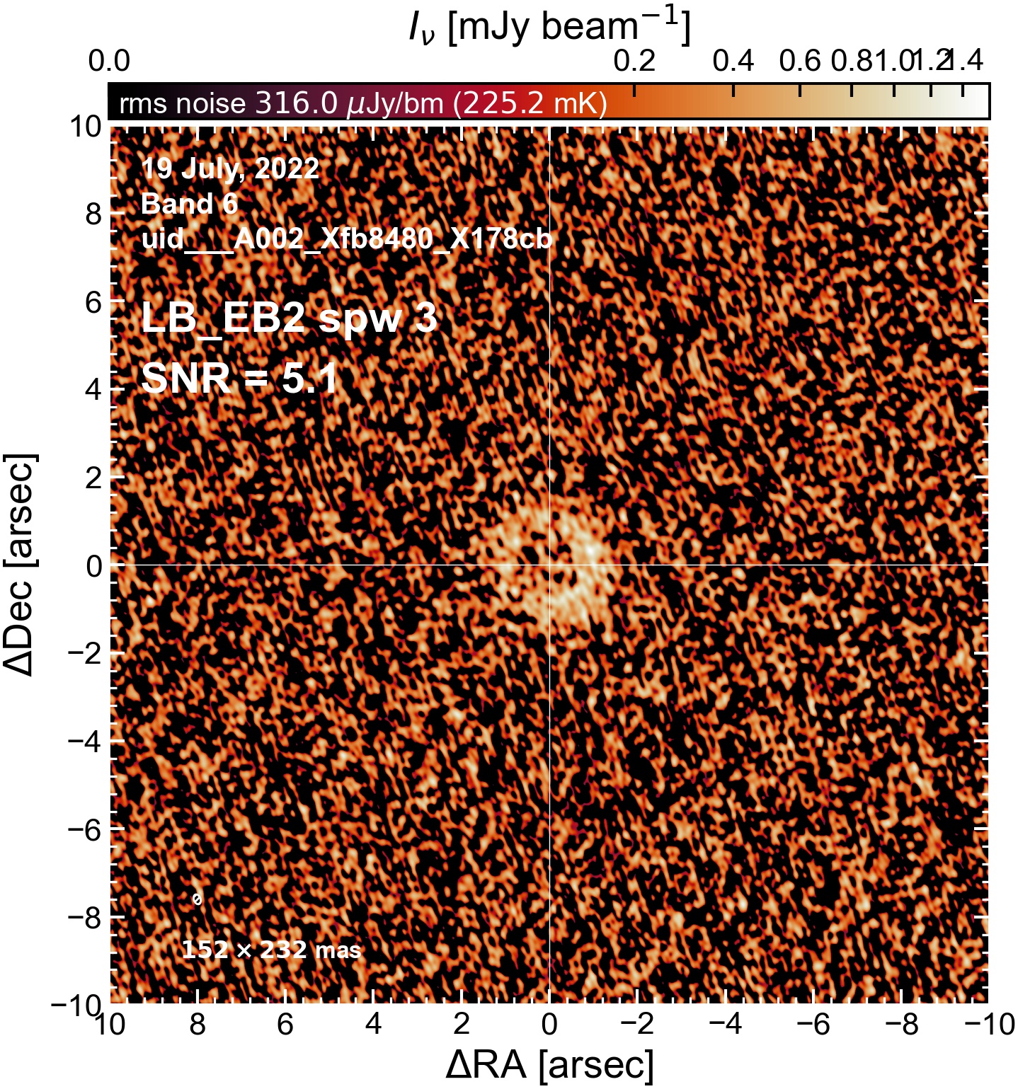
LB EB2#

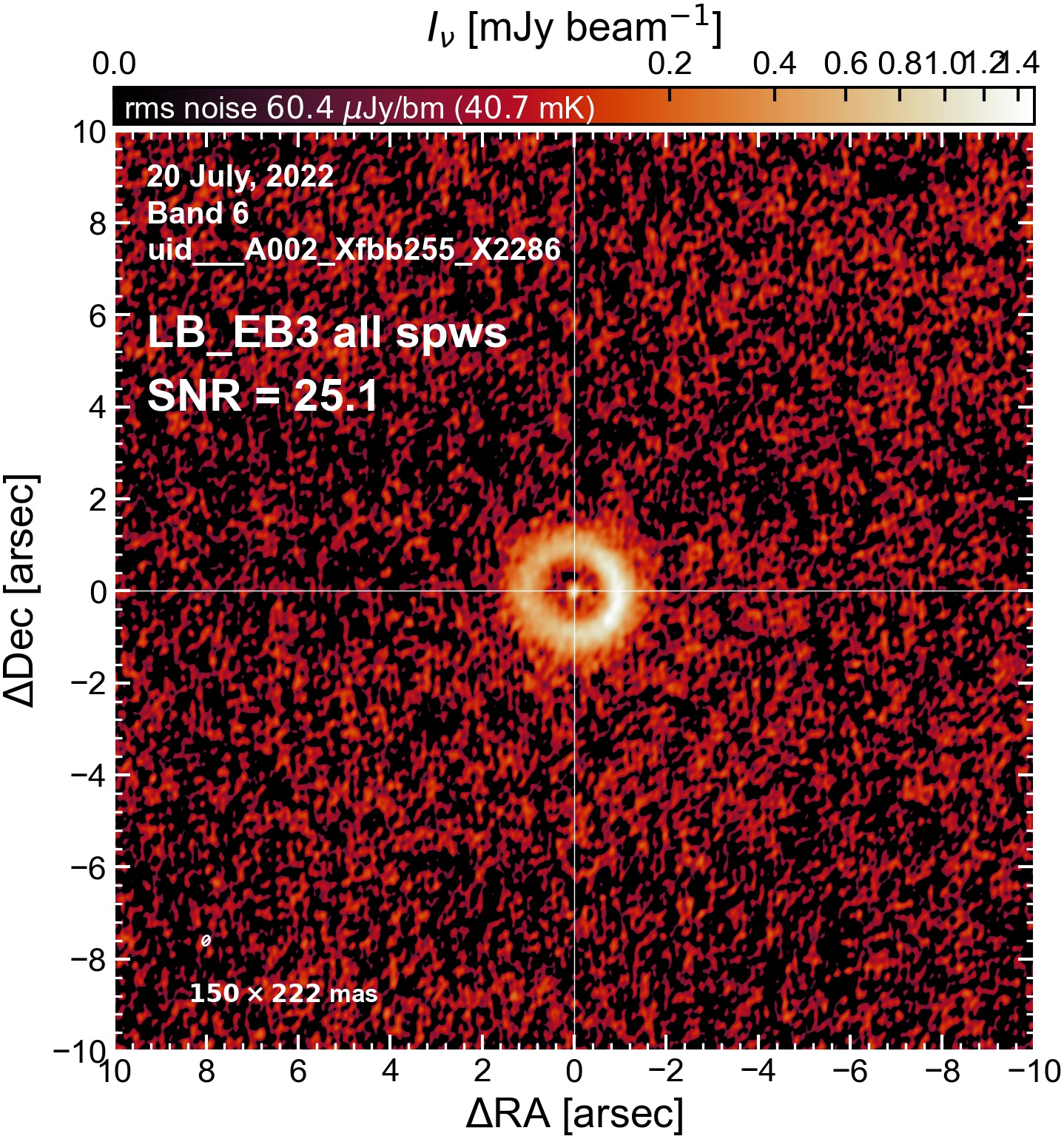
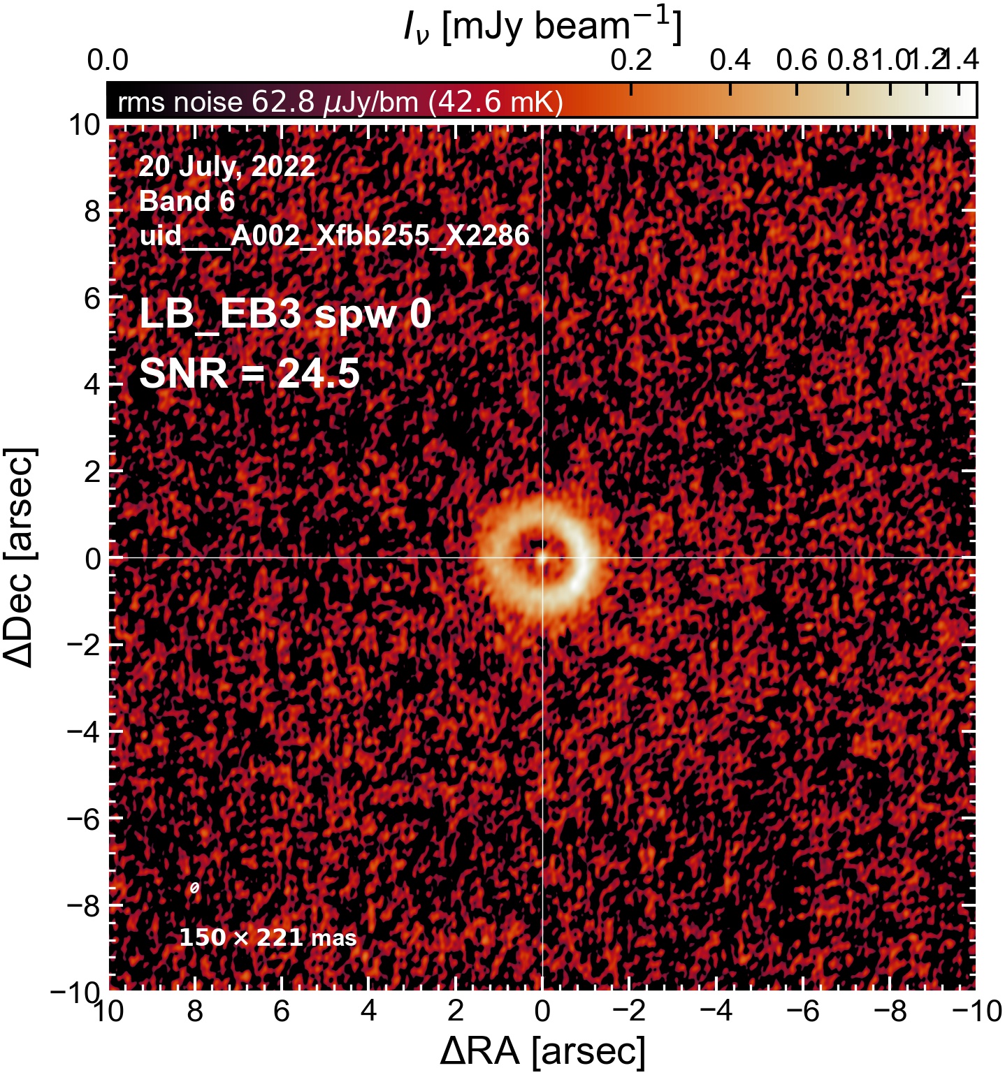
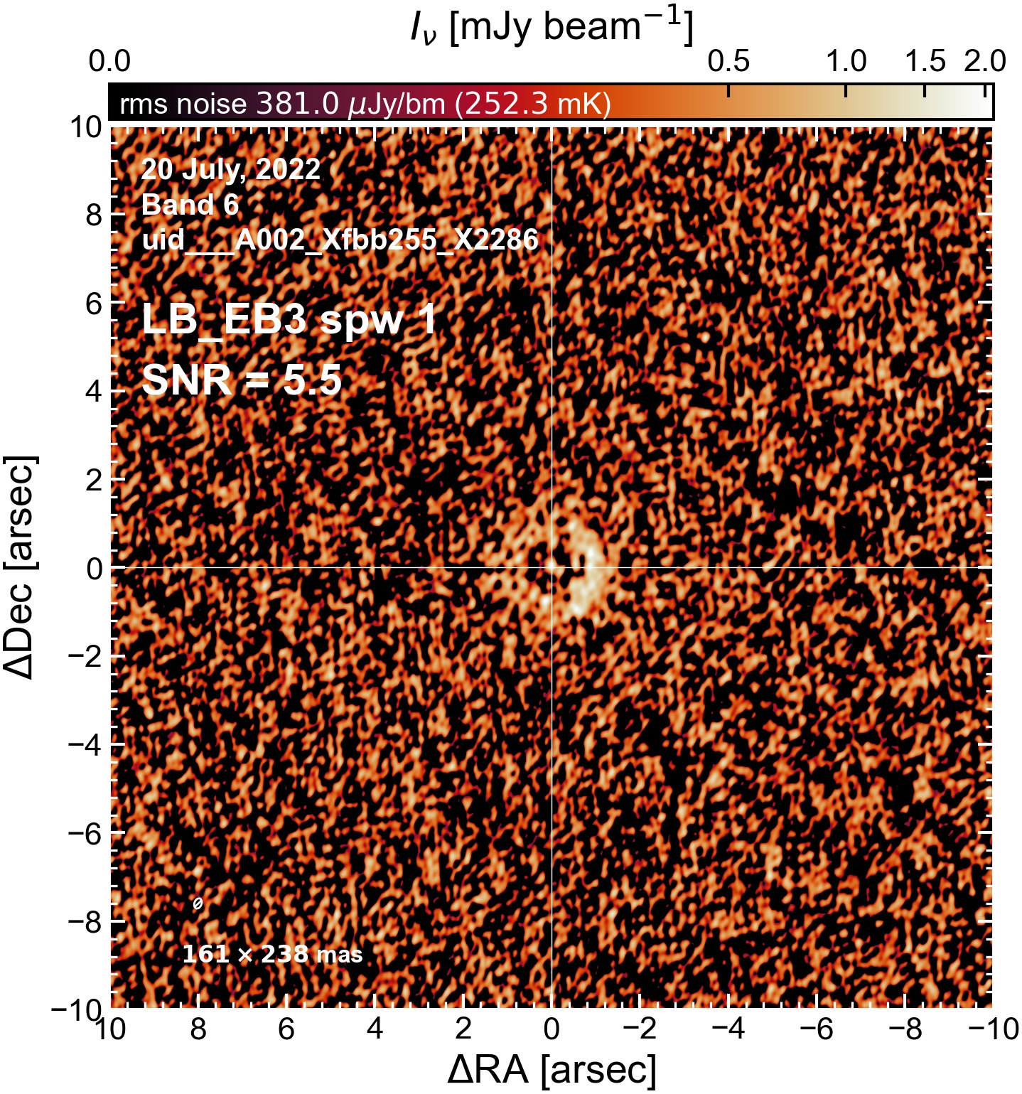
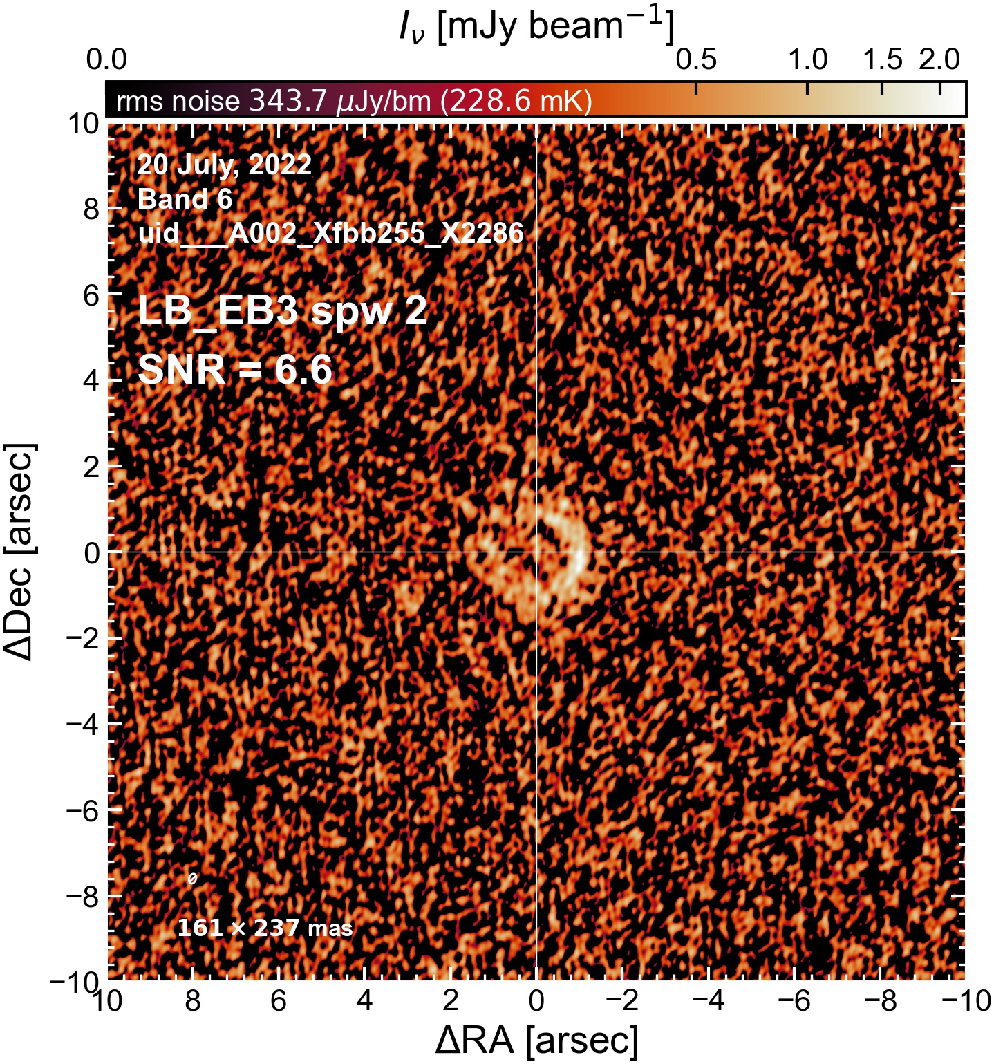
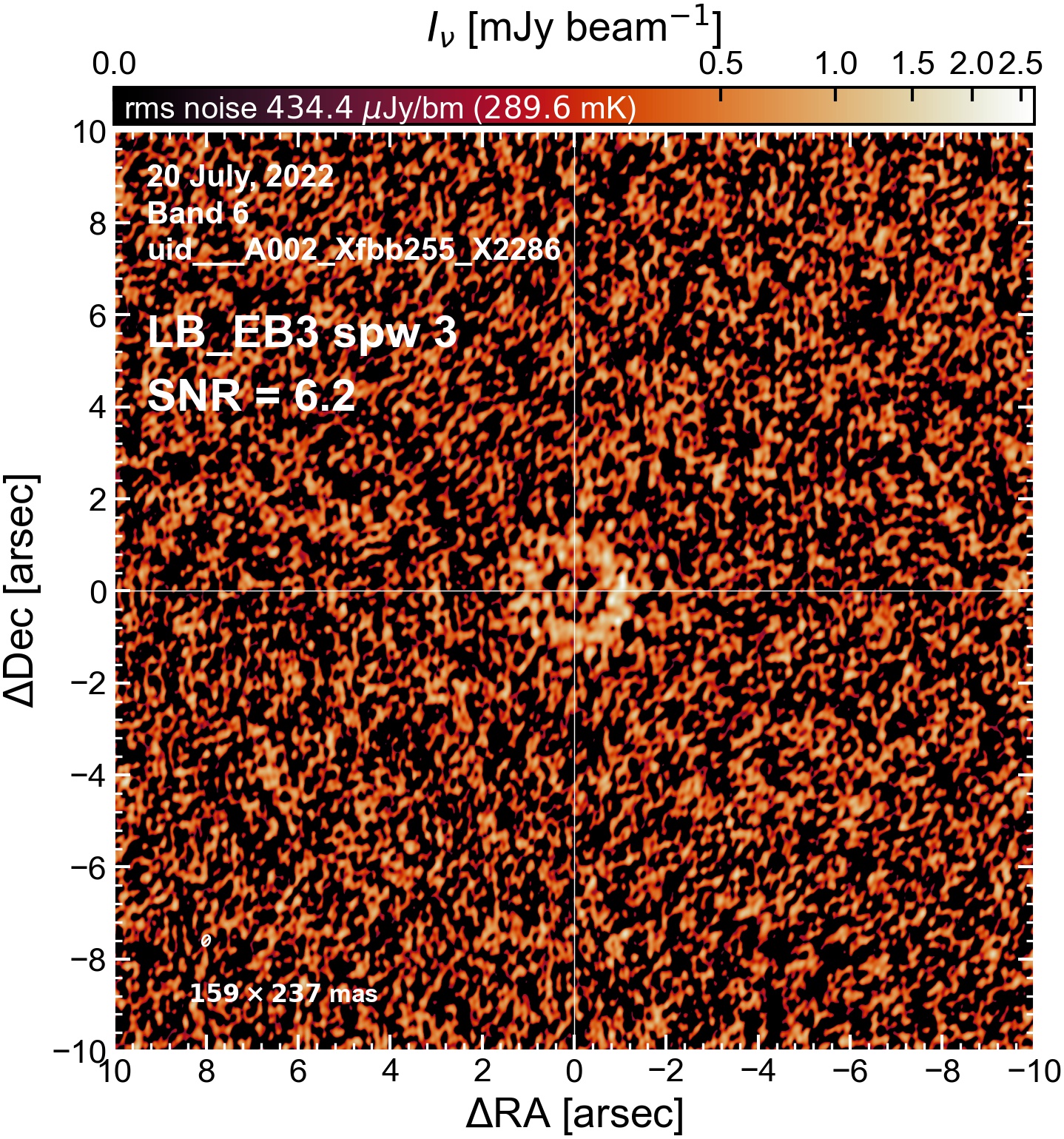
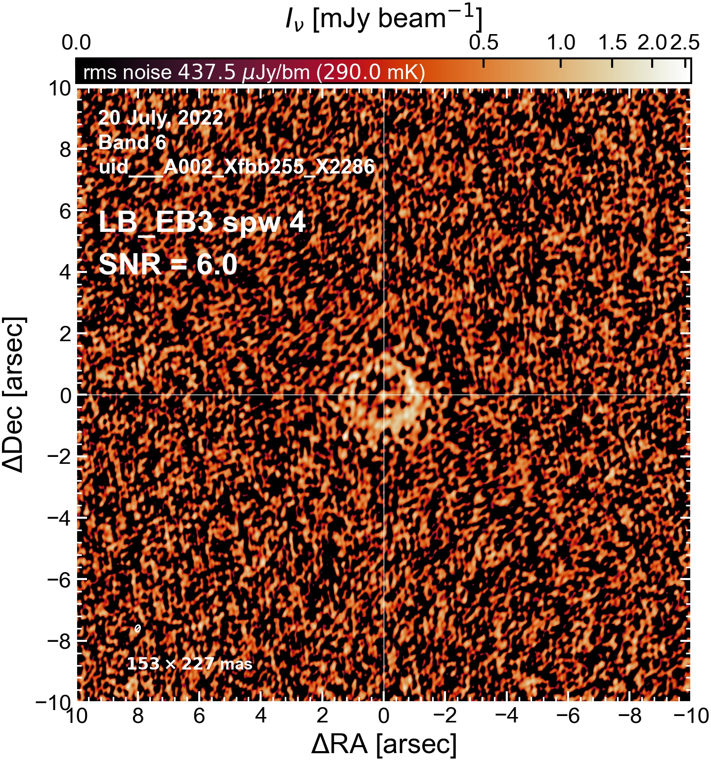
LB EB3#
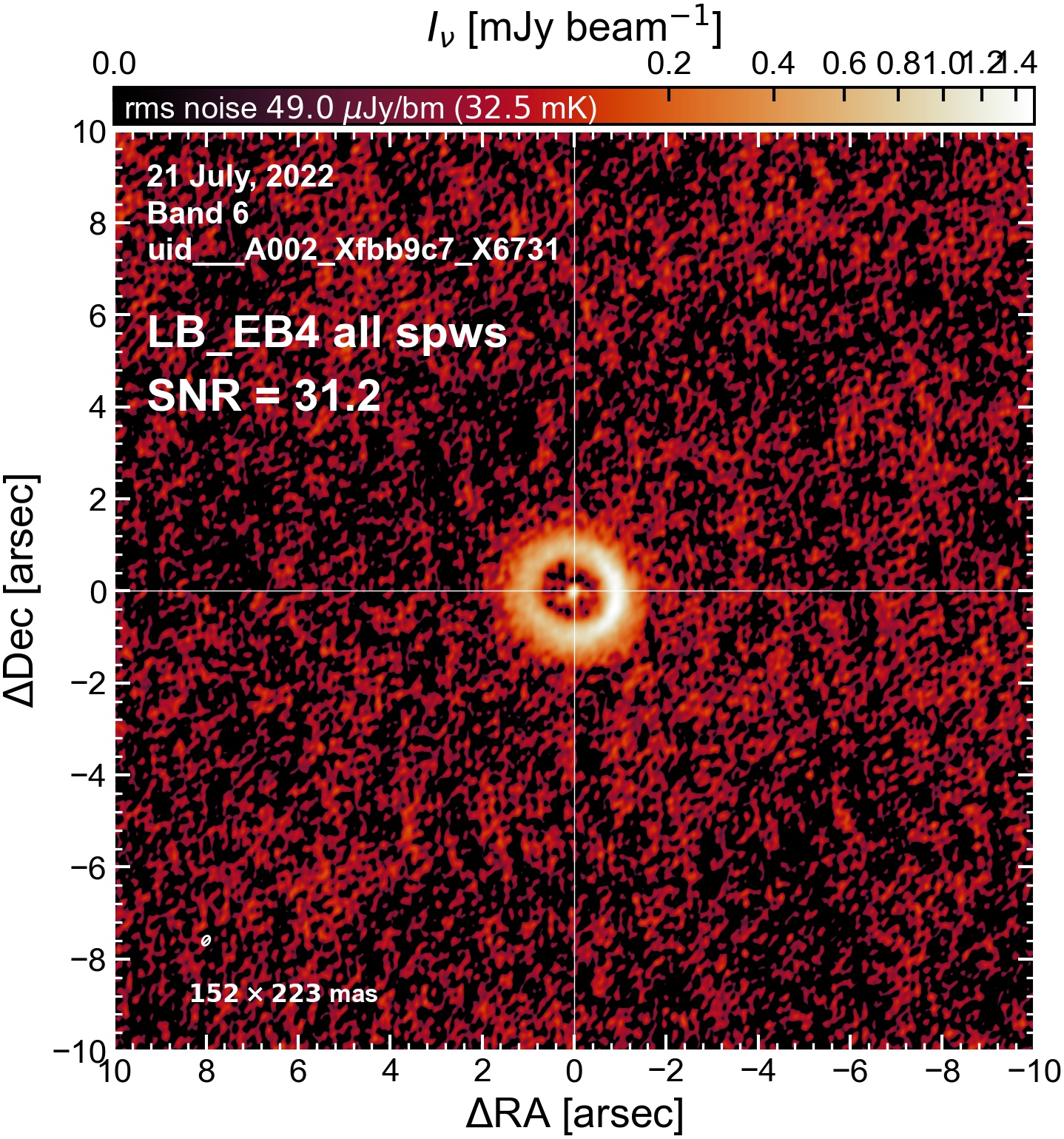
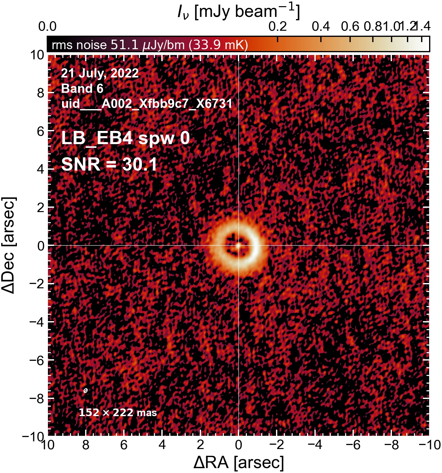
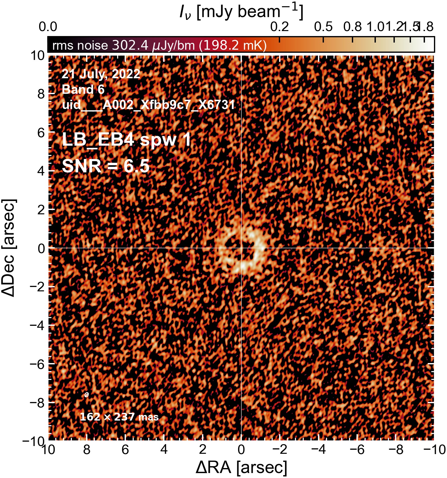
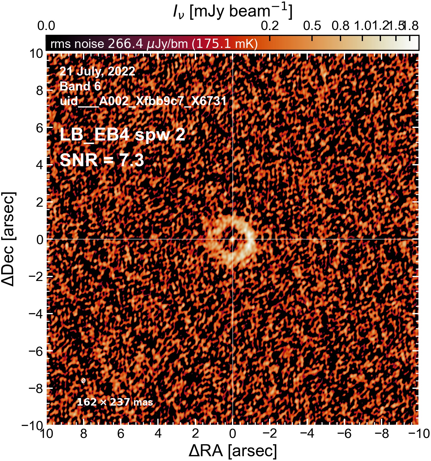
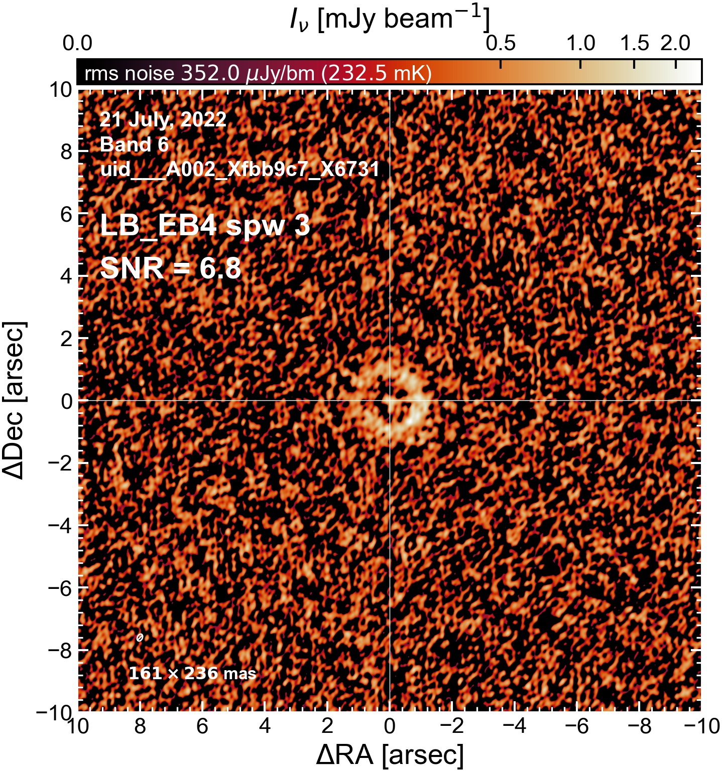
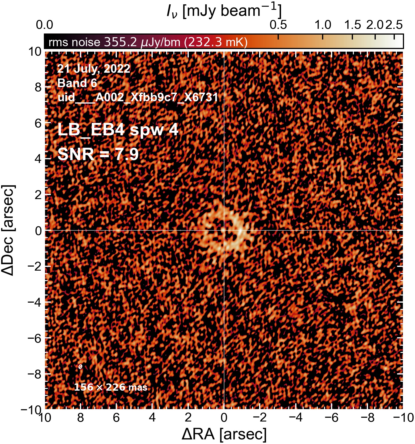
LB EB4#
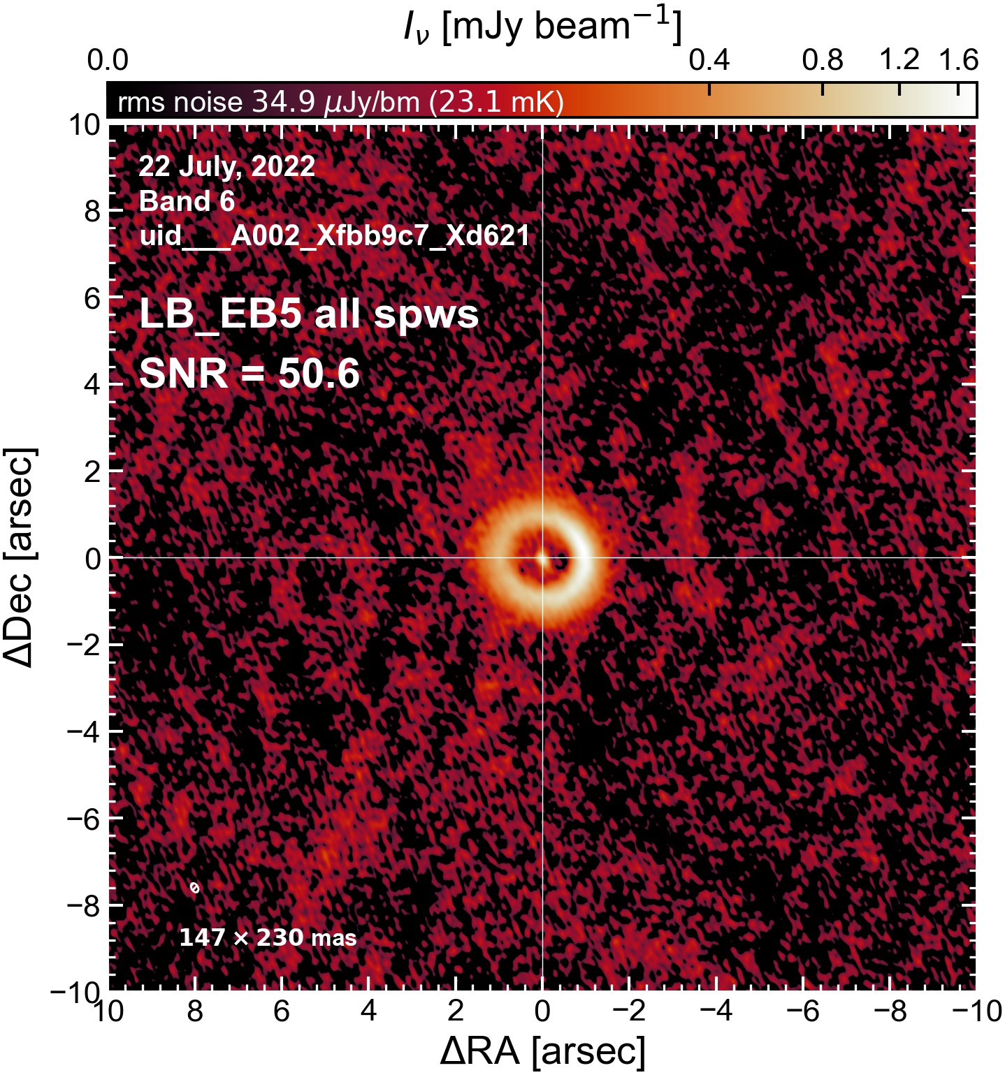
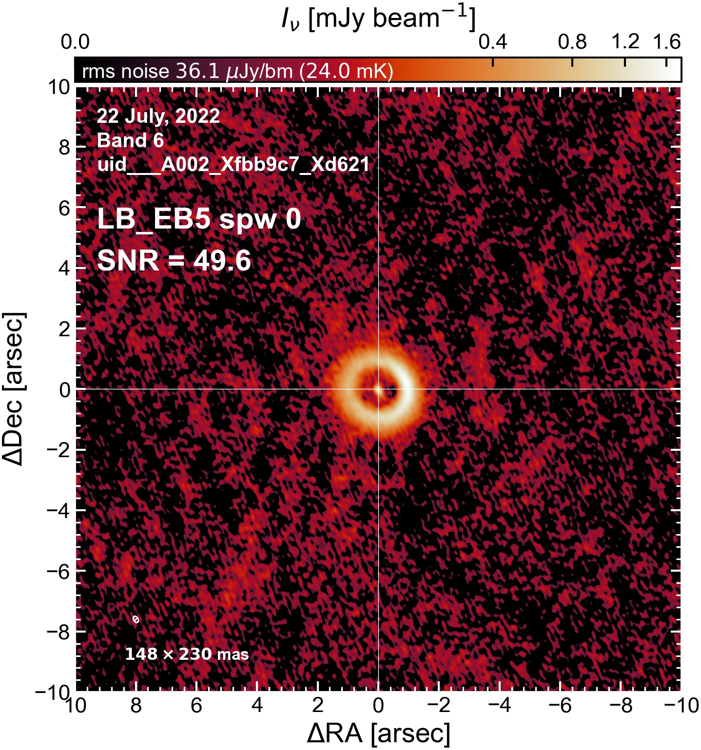
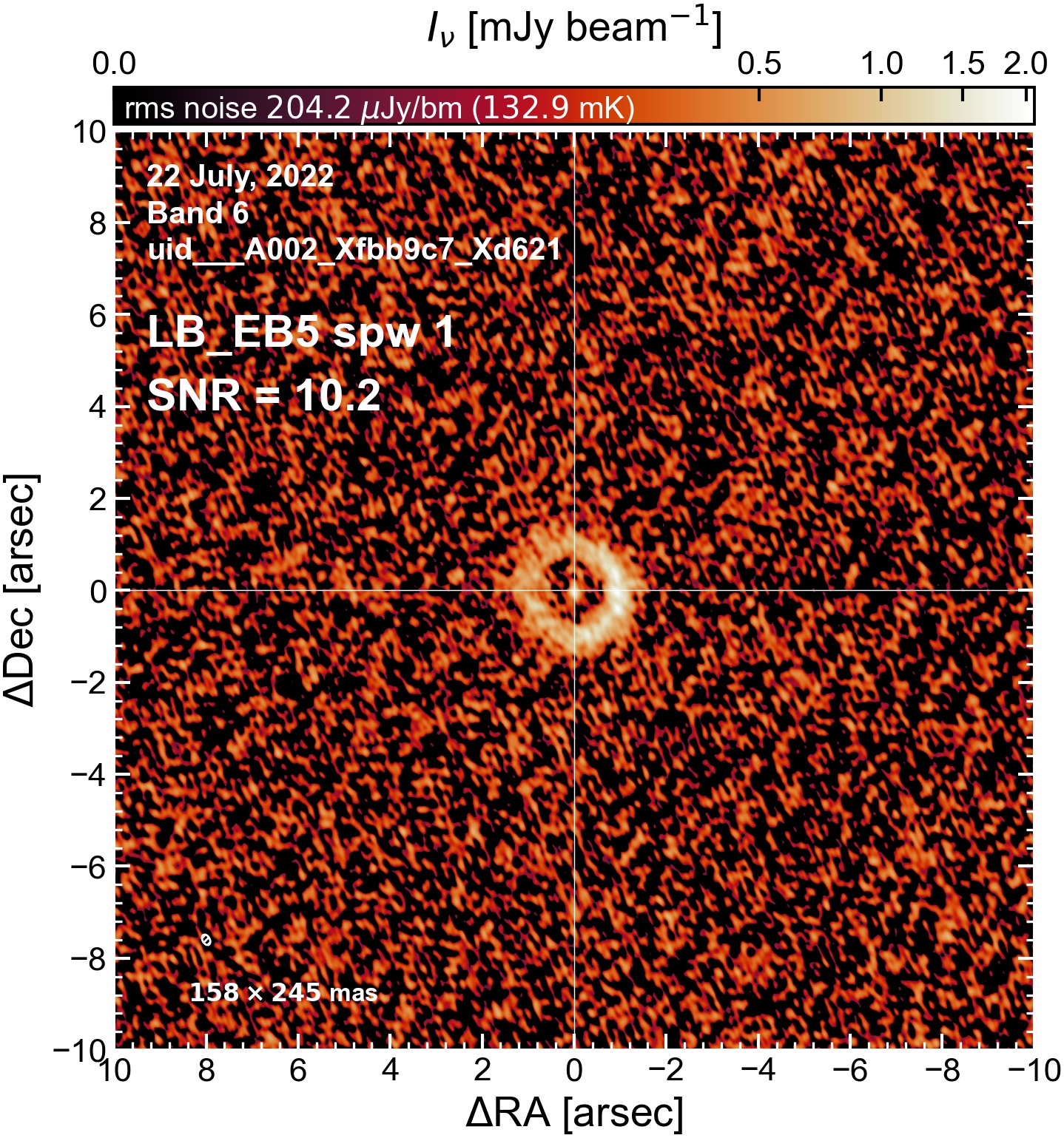
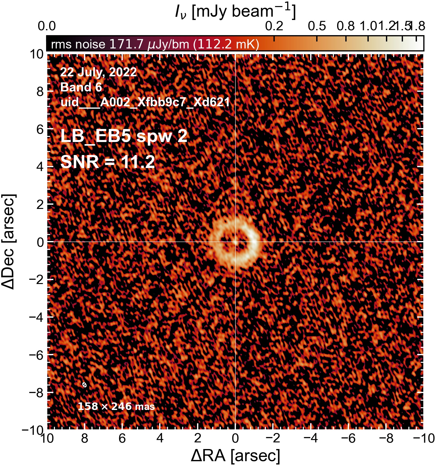
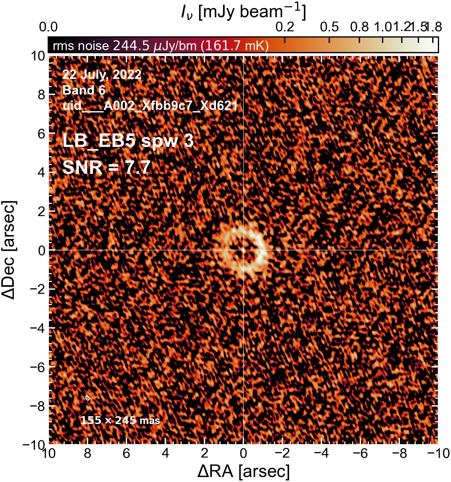
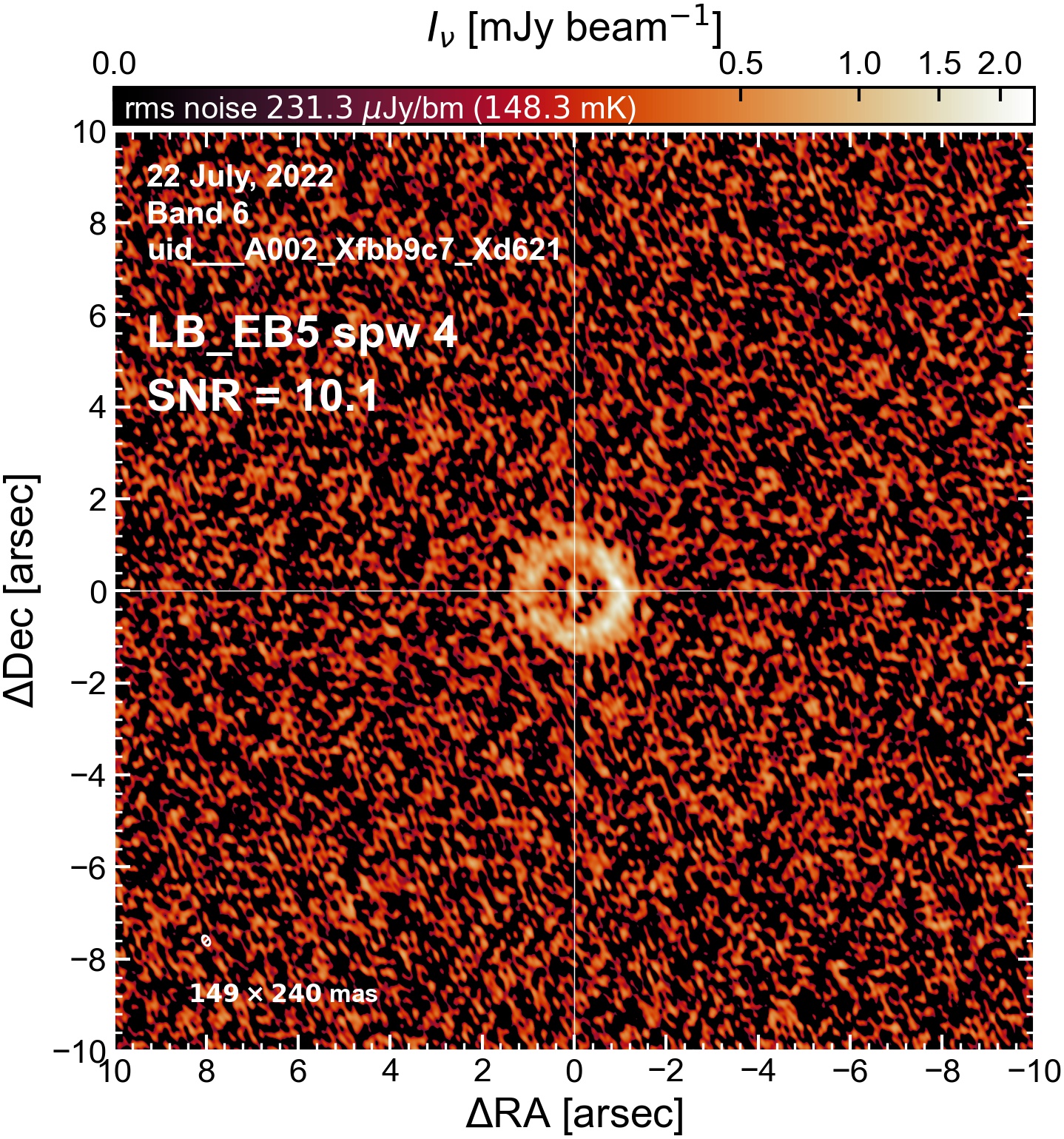
LB EB5#
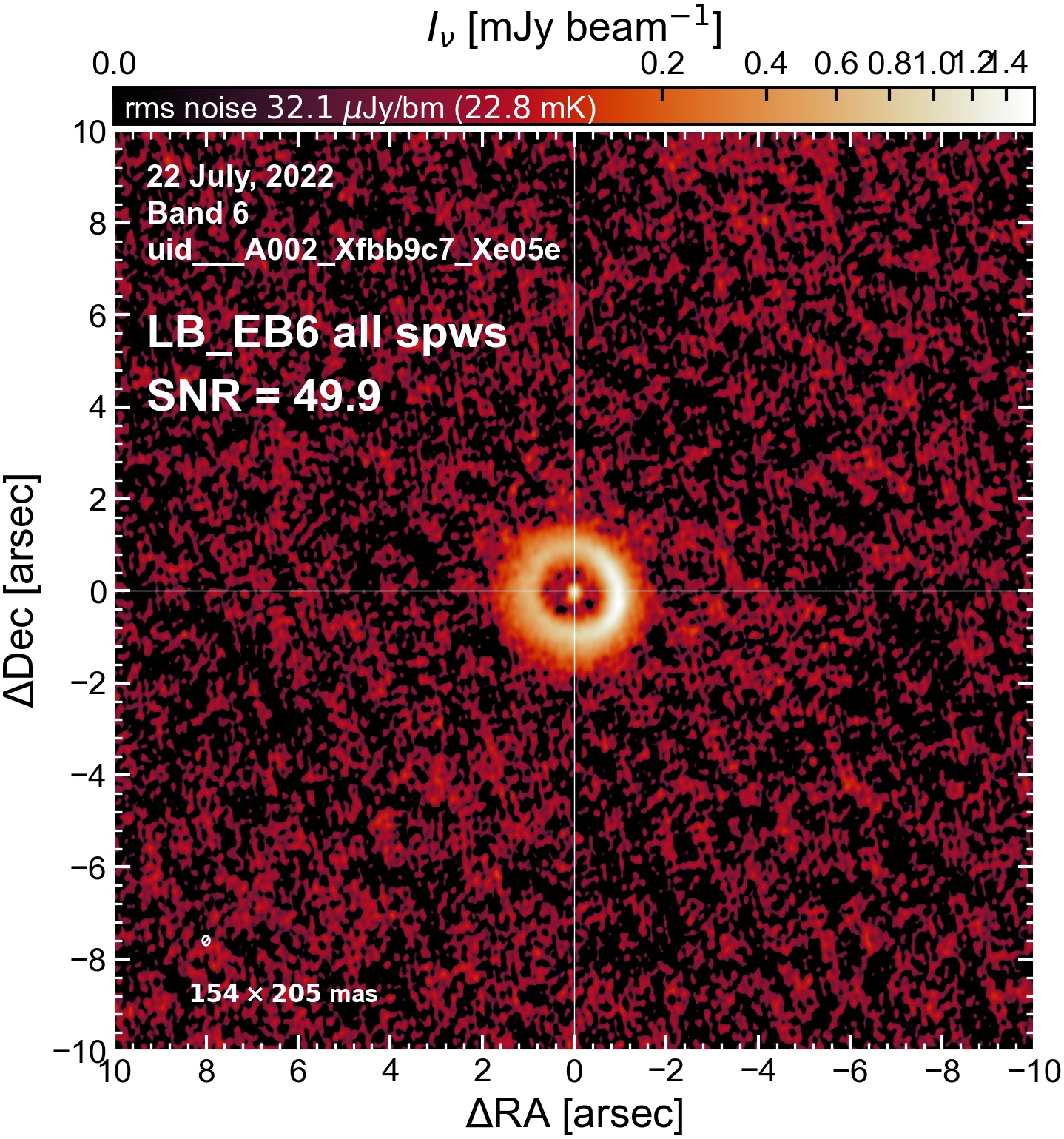
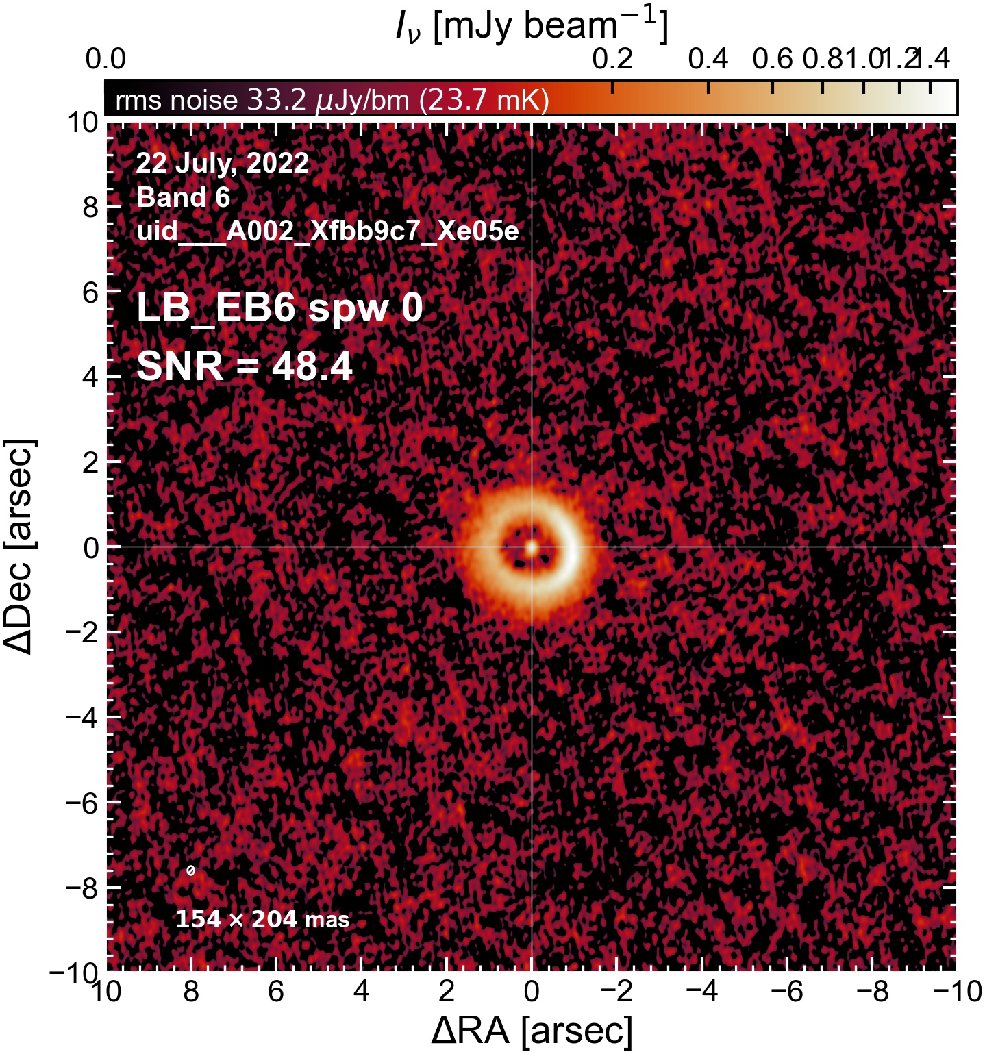
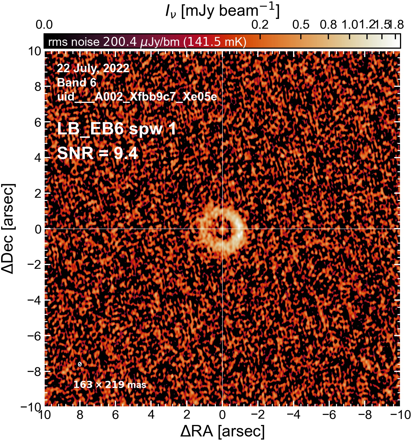
LB EB6#
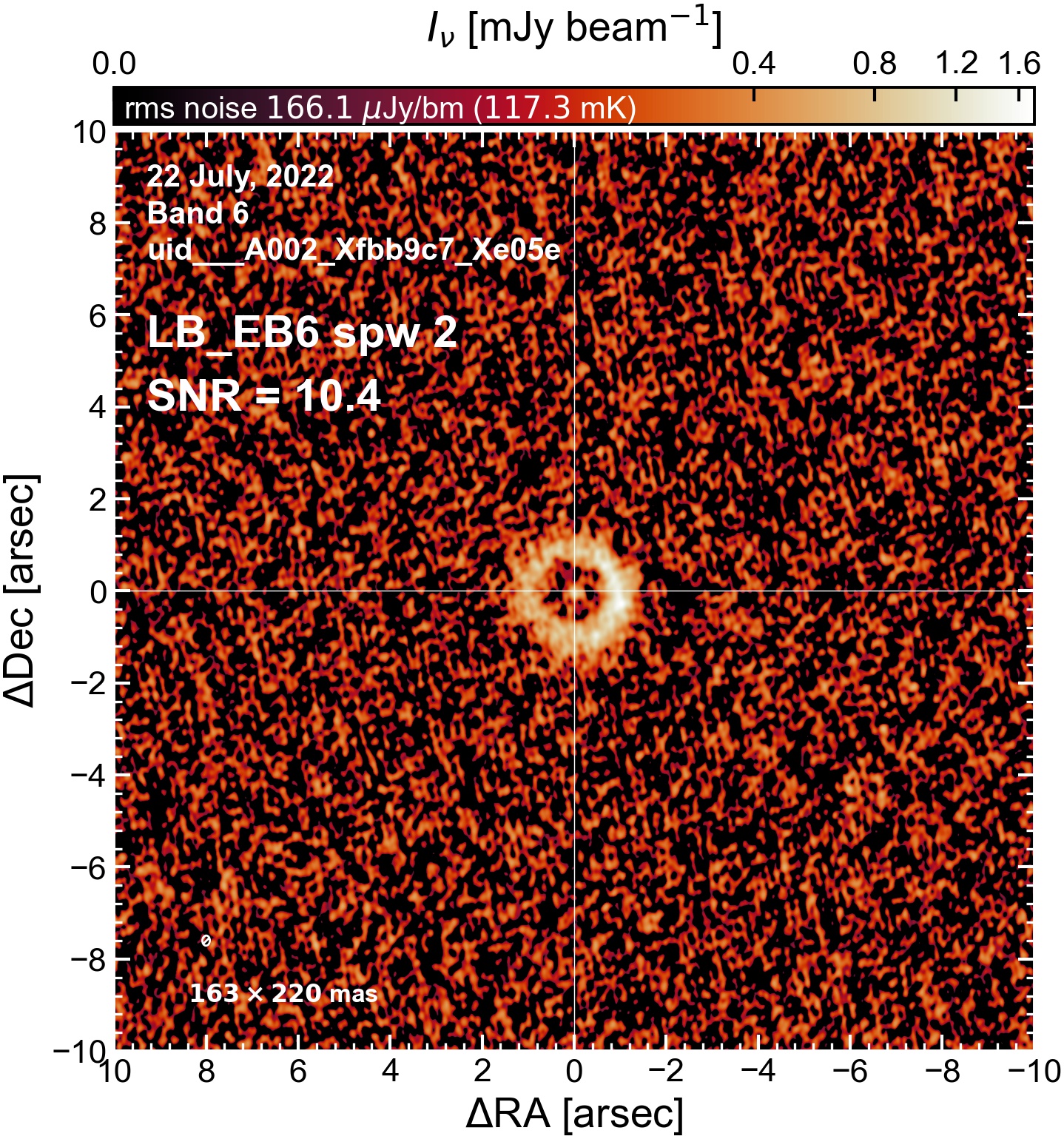
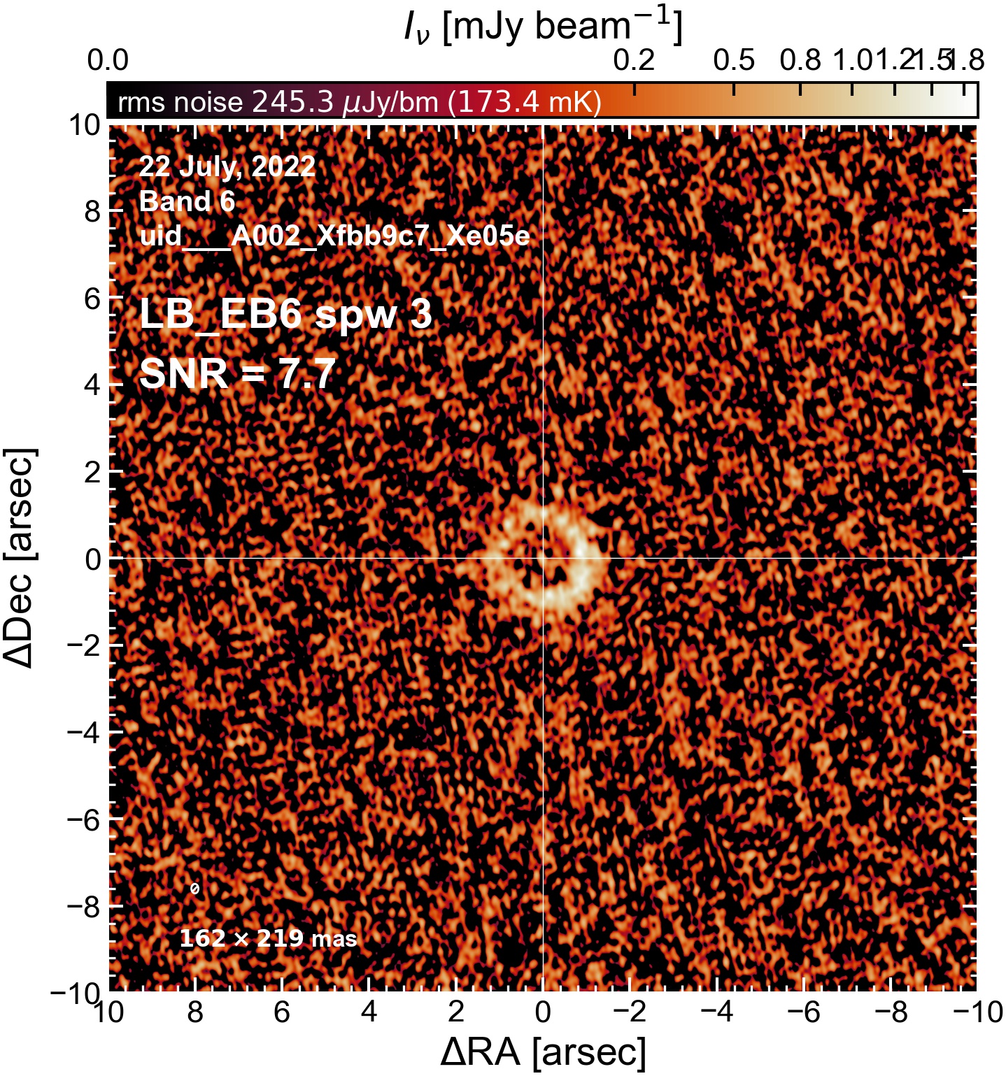
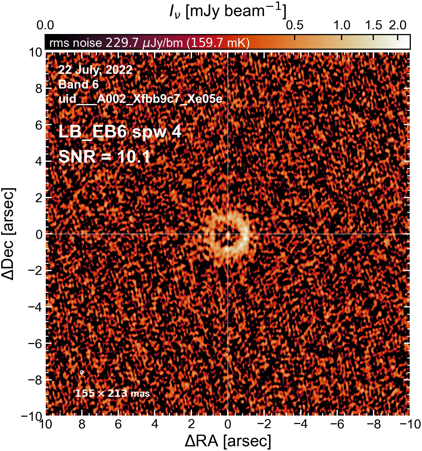
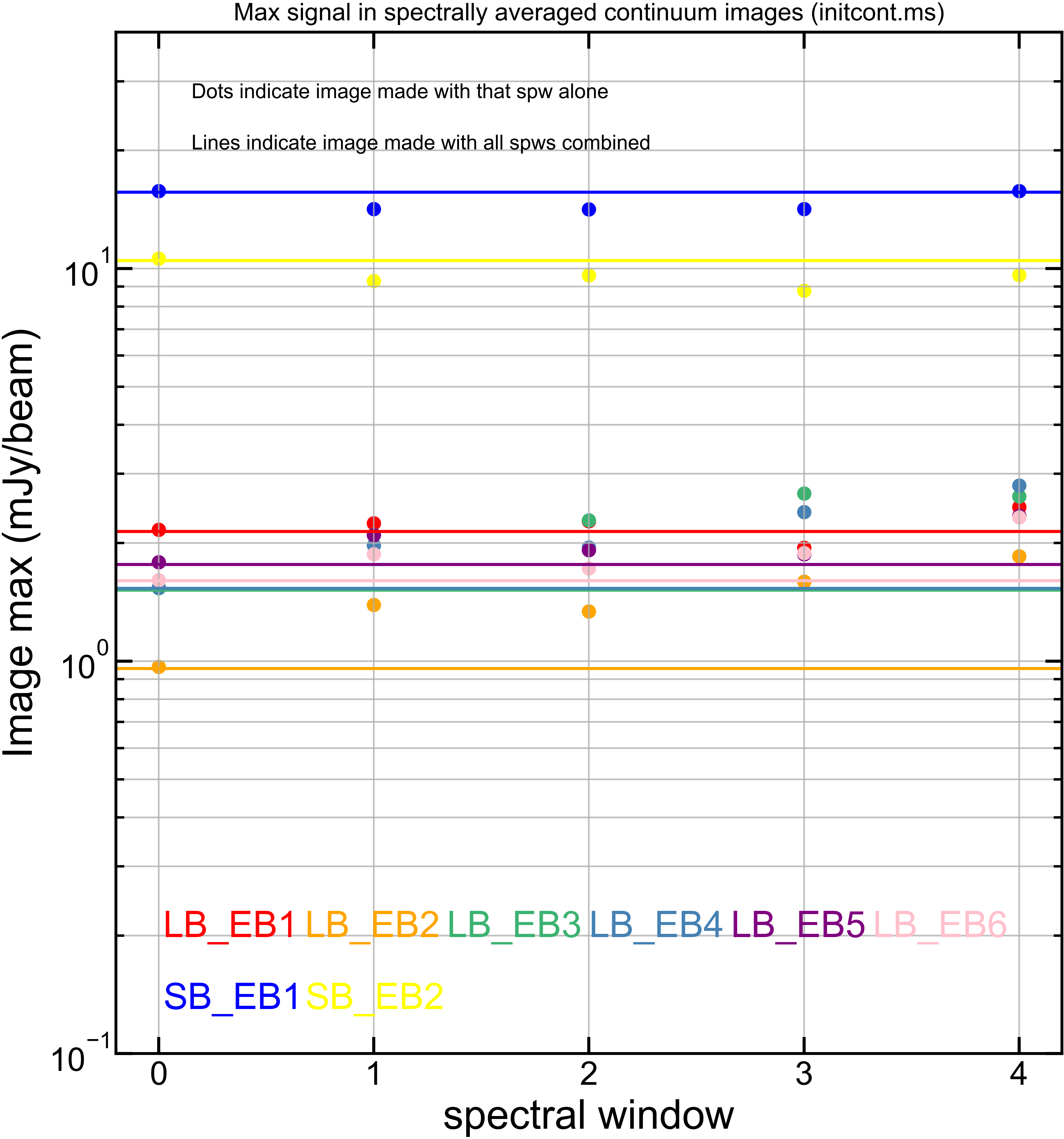
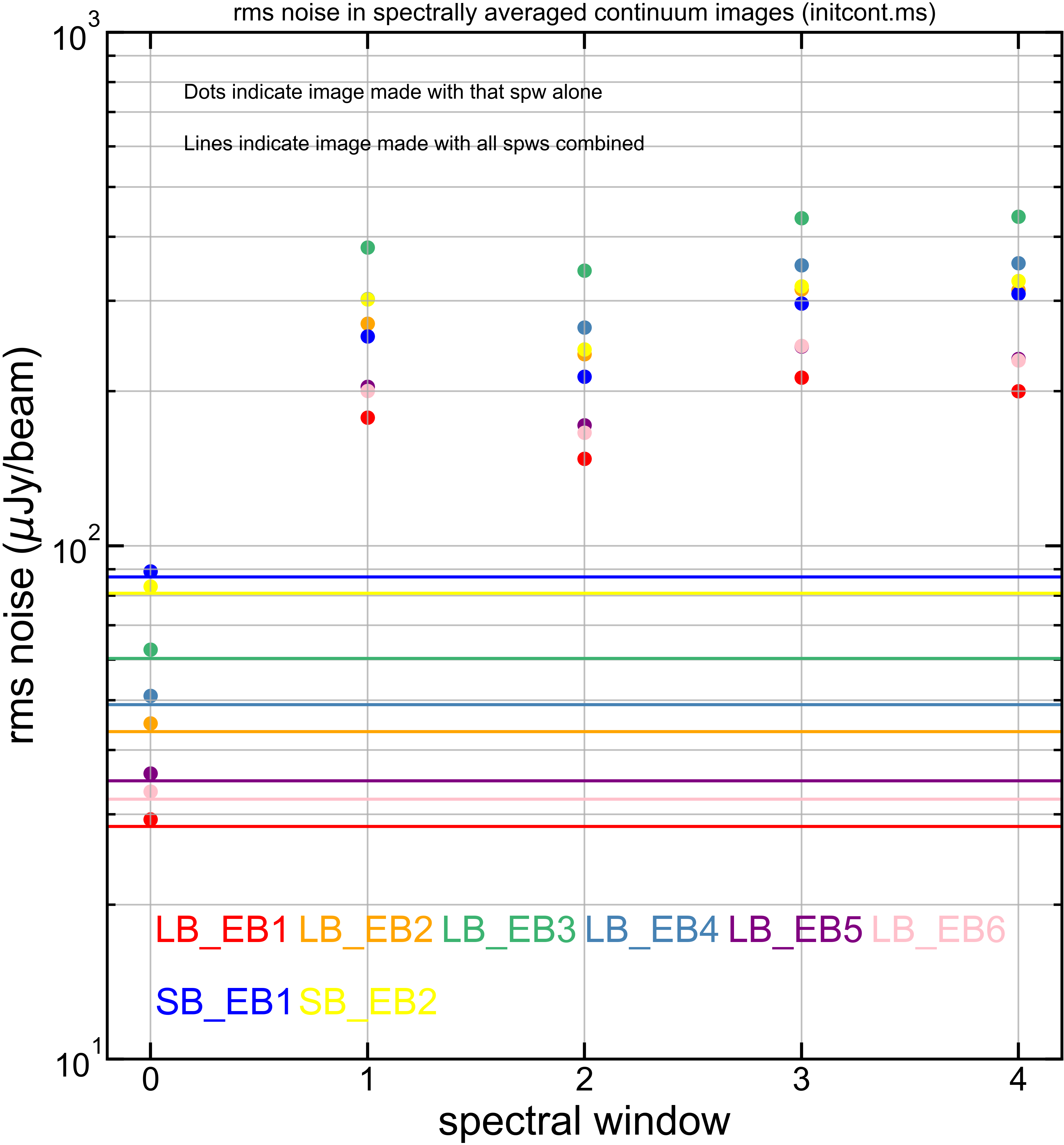
Comparing SNR across EBs#
The following is a summary of the above continuum images (more directly informative for per-spw self calibration). SNR is calculated as SNR = [peak intensity]/[measured rms noise].
A minimum of ~25 SNR is needed for self calibration. So we should be able to do per-spw self cal on the SB execution blocks, but this plot hints that we might not be able to self-cal the LB execution blocks without either concatenating them together, or concatenating them with the SB data.
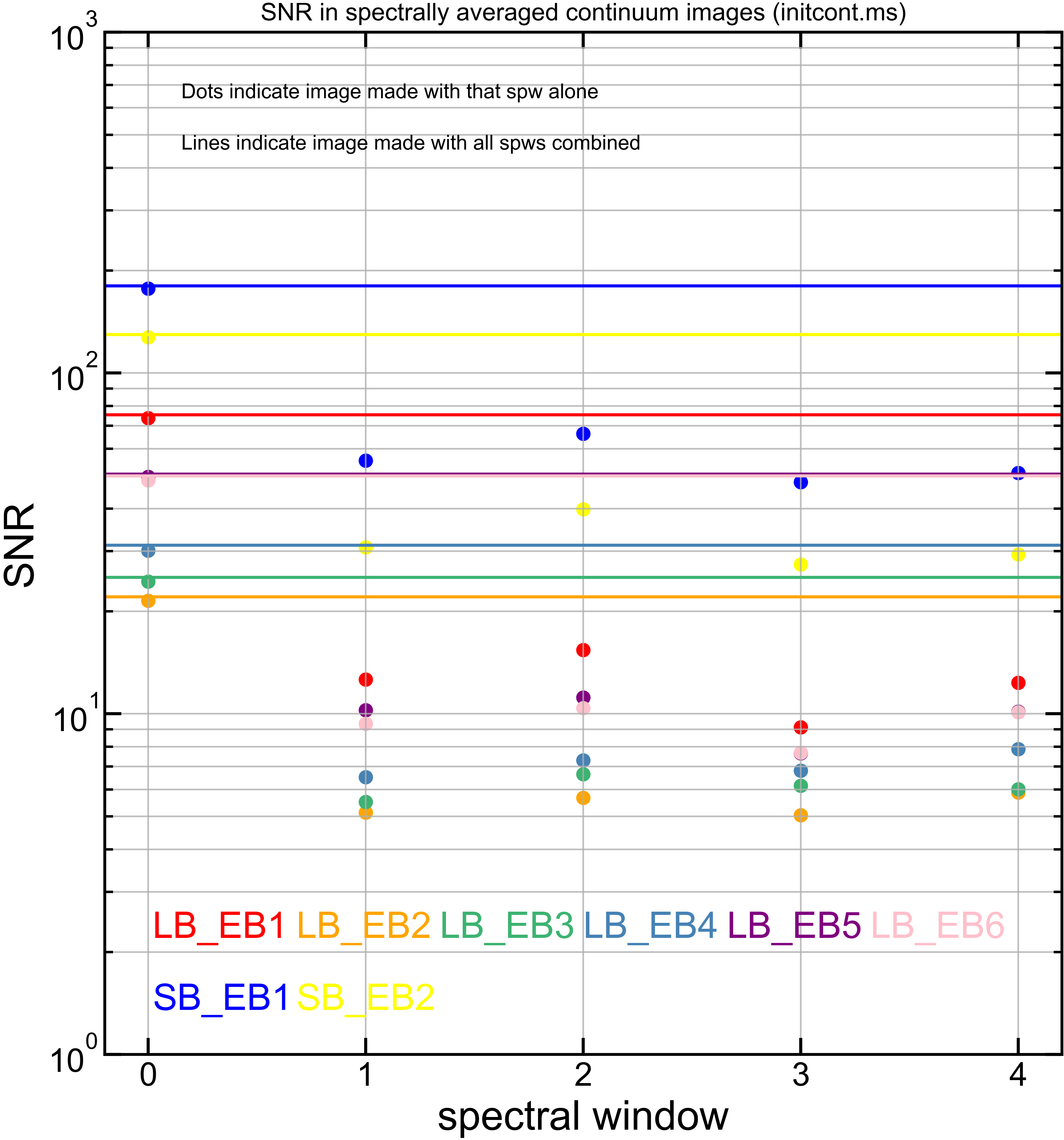
Just for reference, here is the equivalent plots but for each of [peak intensity] and [measured rms noise].