Scripts for Step 3 - Self-calibration of the continuum:

• step3_continuum_selfcal.py # main script

• dictionary_data.py # loads data_dict

• selfcal_utils.py # selfcal functions

Self-Calibration of SB+LB Data

Here, we self-calibrate the long-baseline and short-baseline continuum data together (phase-aligned and concatenated).

Summary of path through self-calibration

Path through LB+SB self-cal. This table portrays the path taken through self-calibration through the choice of parameters in every round. Self-cal “starts” in the third column (“Round p0”) with the tclean task, and then proceeds to the fourth column (“Round p1”) with the gaincal task, and so on. We performed six rounds of phase-only self-cal (“p1”, “p2”, “p3” etc.), and one round of amplitude+phase self-cal (“ap”). In each round, the parameters in the tclean, gaincal and applycal tasks were set as listed in that round’s column. In CASA, setting a parameter to '' means “all” or “nothing”. Rows to look at include solint (the solution interval), calmode (phase or amplitude+phase), combine (note 'spw' is now always combined), and the number of failed solutions (that did not satisfy our SNR requirements). The threshold parameter for the tclean task is not set because we clean interactively.

(selfcal_dict.txt) The bottom few rows keep track of relevant quantities or image metrics as they change over the course of each round. Rows to look at include SNR (improved from 154 to 239), disk flux (slightly decreasing monotonically), and the beam major & minor axes bmaj & bmin (constant as data associated with failed solutions is not flagged out).

Context for choice of solint: Scan lengths within each execution block. For example, the LB EB3 execution block contained 13 scans mostly 181 seconds long, though some were 121 seconds long. Thus, the solint choices of 900s, 360s, 180s, 60s for the LB+SB self-cal roughly correspond to five scans, two scans, one scan, and a third of a scan in the case of the LB data. Integer multiples of 60s were chosen to be harmonious with the LB scan lengths.

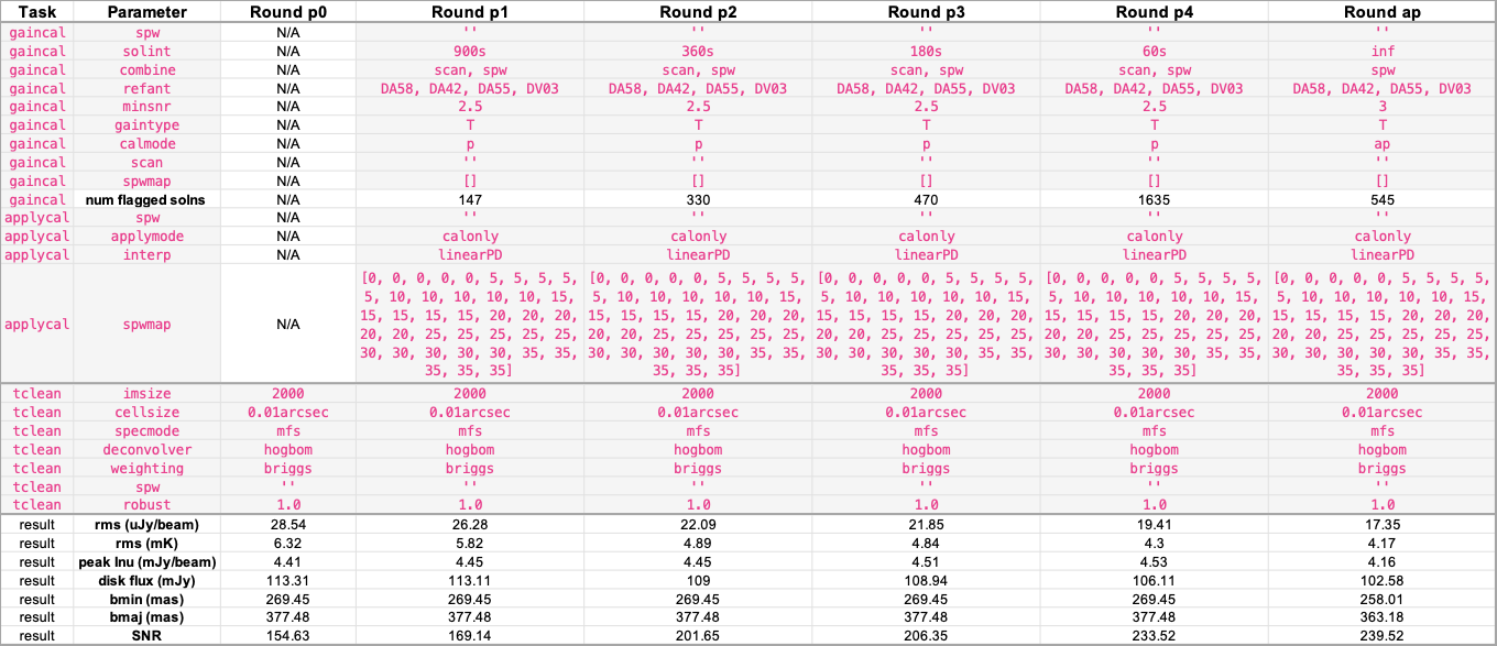
Additional explanation of parameter choices that are different from the SB-only self-cal

In the gaincal task:

• solint: Previously in the SB-only self-cal, we used solints that were nice fractions of the scan lengths. This wasn’t so possible for the LB+SB self-cal, because the LB scan lengths weren’t as consistent. Instead, we reverted to the DSHARP/MAPS solint sequence.

• combine: This time it wasn’t possible to avoid combine='spw' without sacrificing a lot of data. What constitutes “a lot” is subjective, but my sense was that there were too many printouts of flagged solutions (see the the script).

• refant: Again selected using the refant lists generated by the pipeline hif_refant task, shown in the weblog. This time the antenna rankings changed between the different executions, so I calculated an “overall ranking” by multiplying the rank of each antenna in each execution and taking the four with the smallest overall rank.

• minSNR: Same as the SB-only self-cal. Perhaps it’s worth noting though that DSHARP decreased the minSNR to 1.5 for their SB+LB self-cal.

• num flagged solns: There are a lot more flagged solutions in the LB+SB self-cal than there were in the SB-only self-cal, but (!) we also have a lot more data in the SB+LB self-cal.

In the applycal task:

• applymode: Here we are trusting the wisdom of DSHARP and copying them (they switch to applymode='calonly' for the SB+LB self-cal). This applies the calibrations, but does NOT flag the data where no calibration solutions are found. This means we do not lose data (so our beam size does not increase), but we also bring with data that has not been calibrated. CASA warns to use this with extreme caution.

• spwmap: Since the gaincal combine includes SPW in all rounds, we need a spwmap in all rounds.

In the tclean task:

• robust: In my first SB+LB self-cal venture, I used robust=0.5 as before, but there were a lot of flagged solutions. Ryan suggested we can play with the robust parameter. Getting high SNR is important. We can image with a lower robust later for our final images if we want. So for the self-cal, we increase robust to 1.0.

🐛 Error in Calibrater::solve: Mismatch between Solution frequencies and existing CalTable frequencies

I encountered this (documented) error in the gaincal task using CASA 6.2.1:

Current CalTable nchan= 1
Current CalTable freq = [224698702714]
Current Solution nchan= 1
Current Solution freq = [224698702714]
Diff = [6.103515625e-05]
2022-12-08 21:08:52	SEVERE	Calibrater::solve	Caught exception: Mismatch between Solution frequencies and existing CalTable frequencies for spw=35
2022-12-08 21:08:52	SEVERE		Exception Reported: Error in Calibrater::solve.
2022-12-08 21:08:53	SEVERE	gaincal::::casa	Task gaincal raised an exception of class RuntimeError with the following message: Error in Calibrater::solve.
2022-12-08 21:08:53	SEVERE	gaincal::::casa	Exception Reported: Error in gaincal: Error in Calibrater::solve.

To avoid this bug, it was necessary to switch to CASA 6.4.1 at this point in the reduction process.

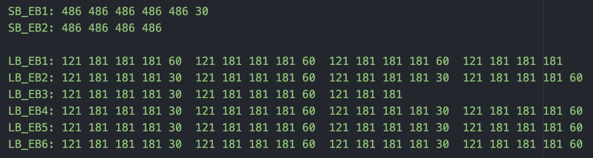
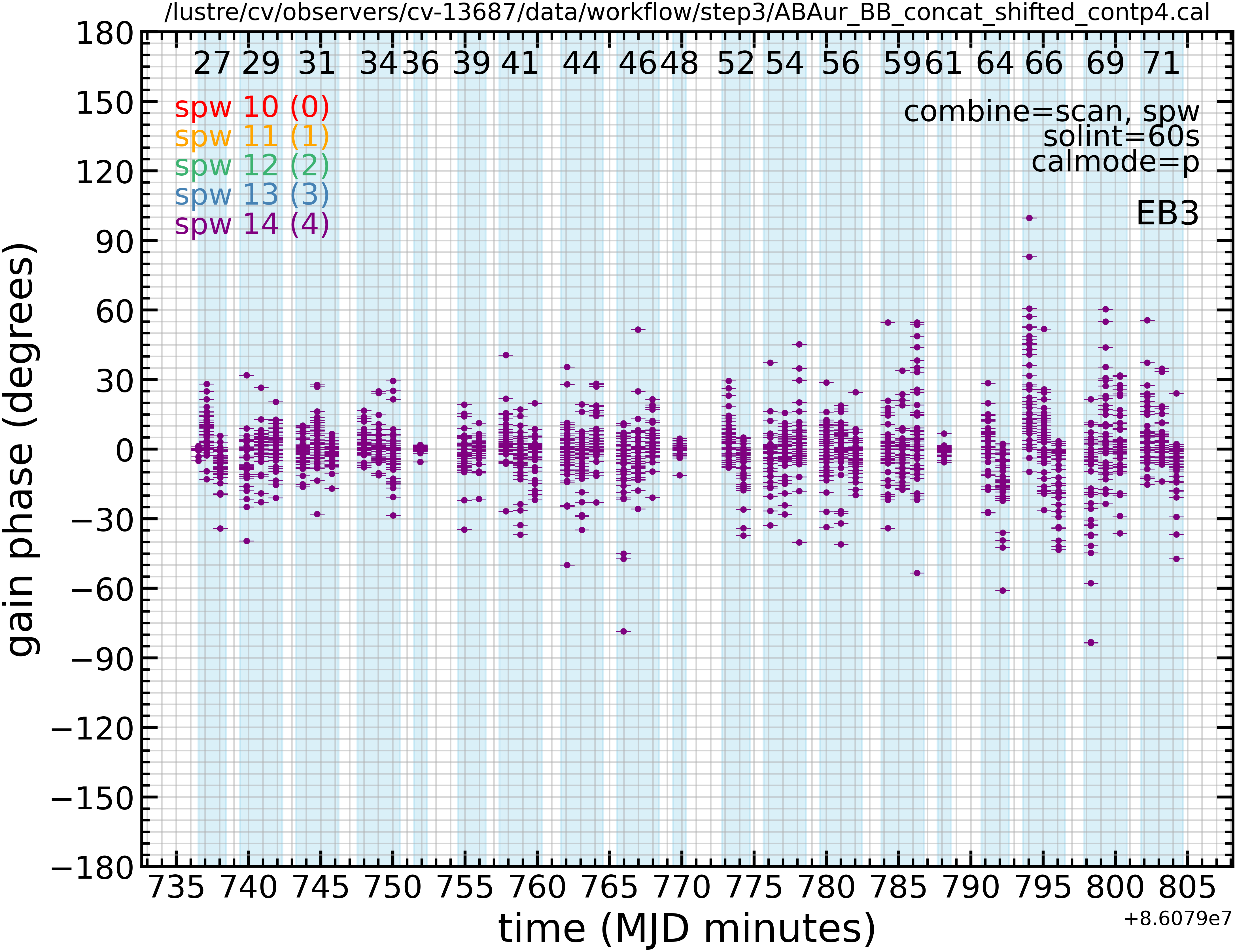
Achieved phase solutions as a function of time and antenna (the calibration tables)

All of SB EB1, SB EB2, LB EB1, LB EB2, LB EB3, LB EB4, LB EB5 and LB EB6 were self-calibrated together. The following plot shows the gain phase solutions as a function of time for a single EB and a single self-cal round.

Self-calibration solutions for LB EB1 (round “p4”). Gain phase as a function of time. Blue shaded regions denote the target scans. The legend says “EB3” because in the combined SB+LB measurement set, the SB EBs take the index of 1 and 2 (so LB EB1 becomes SB+LB EB3). Since all SPWs are combined, points are coloured the same colour (happens to be purple).

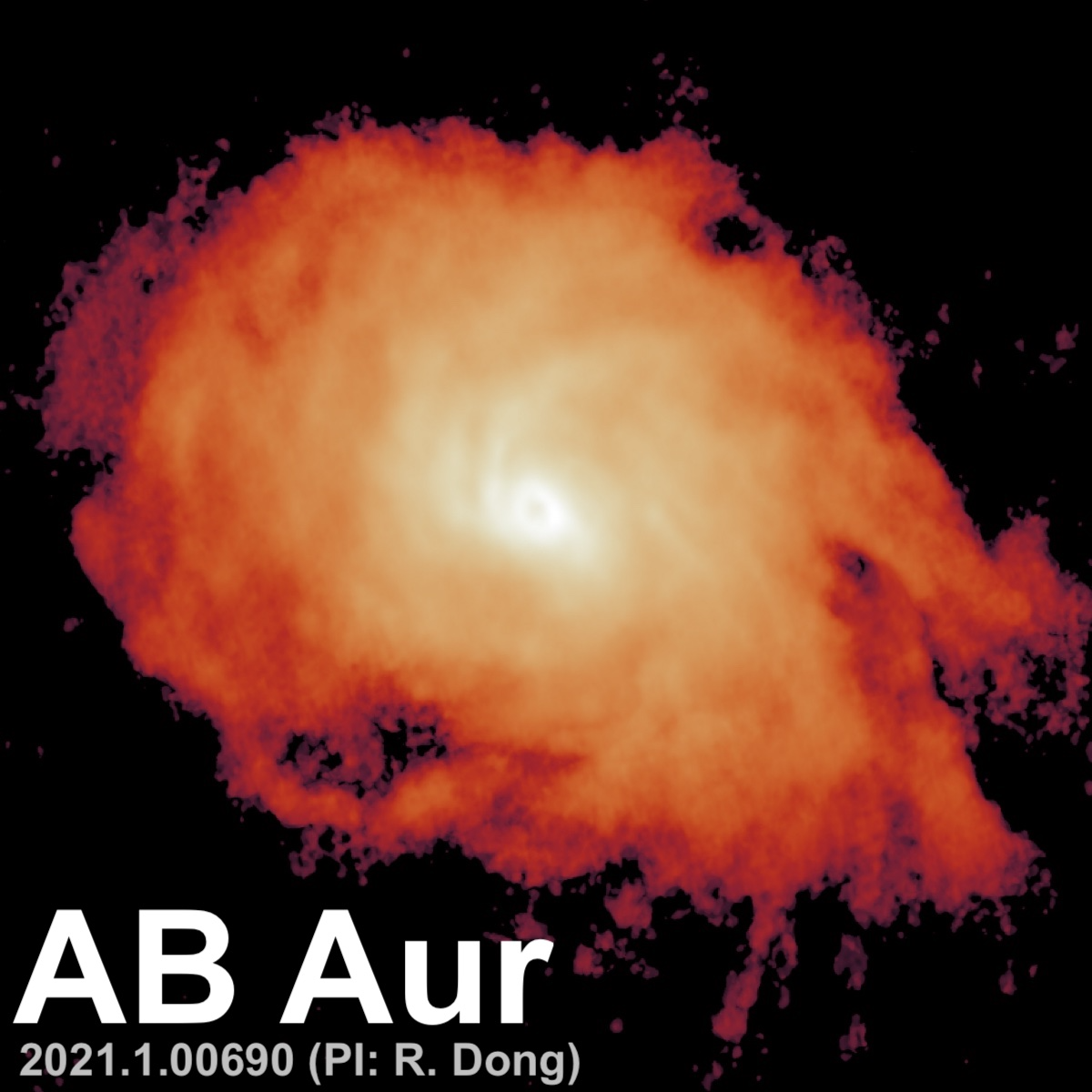
Images made after each round

The following movie shows the continuum image achieved after each round of self-cal (with a large colour bar stretch to exaggerate faint emission).

Continuum image achieved after each round of LB+SB self-cal. Things to notice: (1) the SNR increases; (2) the images visually improve; (3) the beam does not get bigger.

The results, before and after

A gif blinking between our initial image (round “p0”) and our final image (round “ap”). We achieve a decrease in rms noise by a factor of 1.6. The peak intensity decreases by about 0.3 mJy/beam. The SNR improves by a factor of 1.5. The outer ring becomes more well-defined. The inner cavity appears emptier; the inner disk appears unchanged.