Tutorial 4: Manual Self-Calibration#
ALMA Primer Video Series: An Introduction to Self-Calibration
This script was written for CASA 6.6.4.34
Source: First Look at Self Calibration (CASA Guide)
https://casaguides.nrao.edu/index.php/First_Look_at_Self_Calibration_CASA_6.5.4
Adapted for ALMA Data Processing Workshop @ University of Victoria
J. Speedie (jspeedie@uvic.ca) October 2024
Dataset: TW Hya calibrated continuum measurement set (435 MB)
twhya_calibrated.ms.tar (Download)
Your working directory should look like:
TUTORIAL4 >> ls
script_manual_selfcal.py
twhya_calibrated.ms.tar
Untar with:
tar -xvzf twhya_calibrated.ms.tar
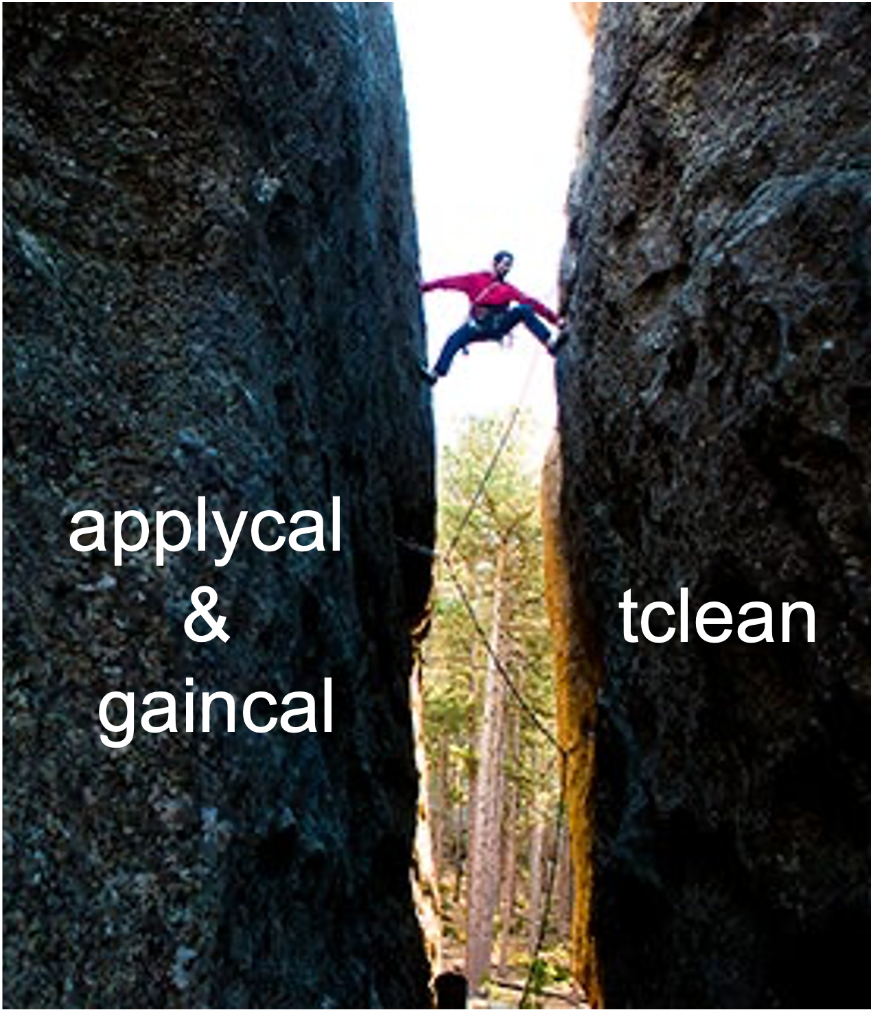
A selfcal meme#
Self calibration is like shimmying up a chimney:
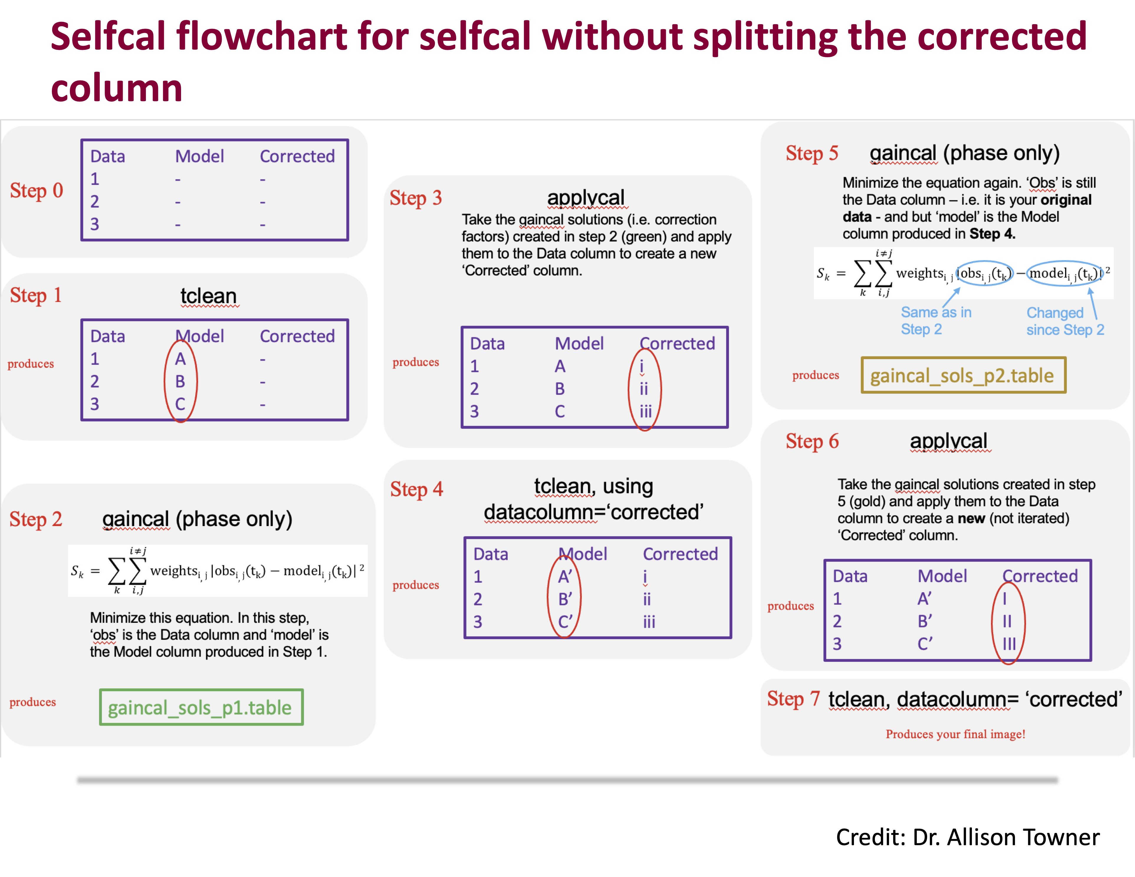
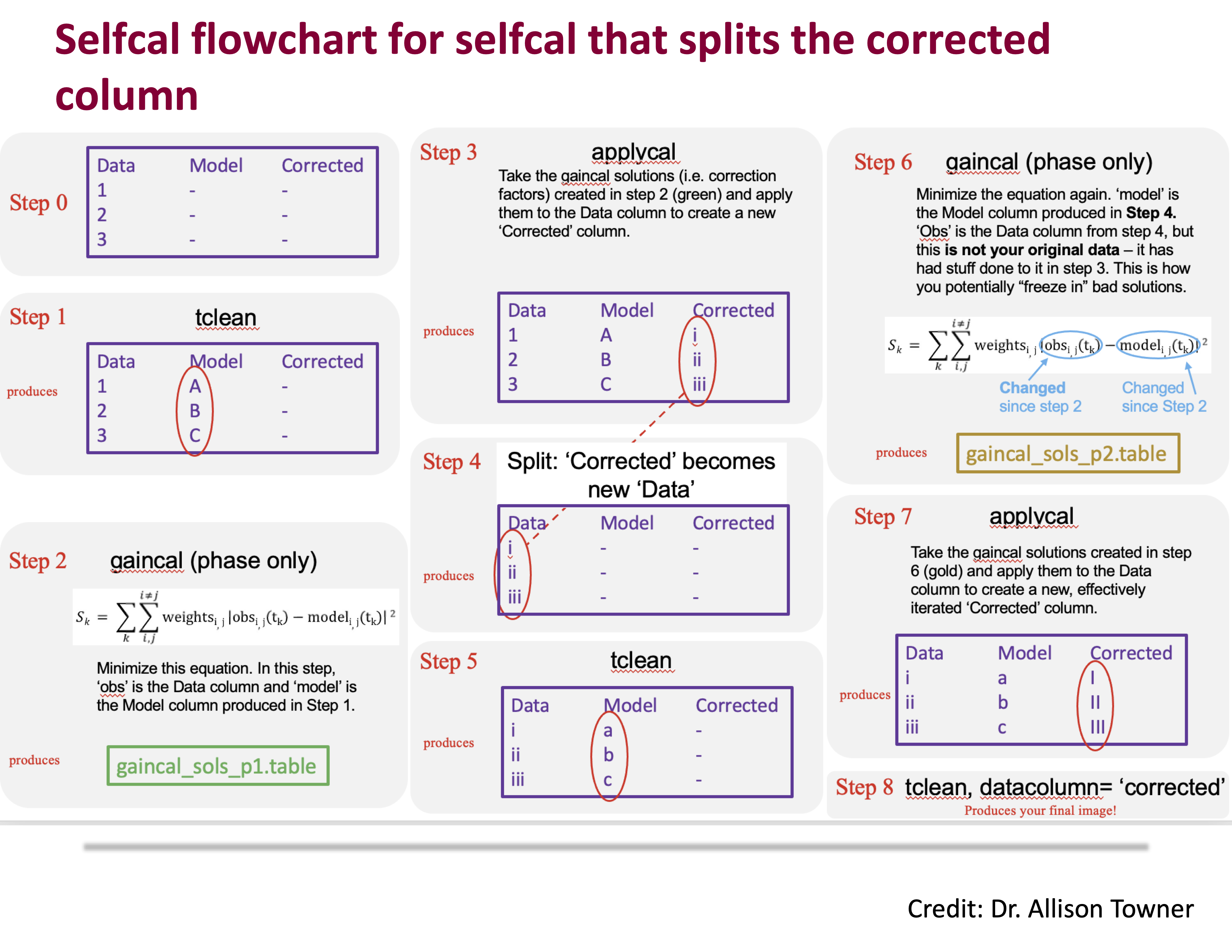
Flowcharts by Allison Towner#
Self calibration flowchart for selfcal without splitting the corrected column:
Create the initial model (Step 1)#
(Here we clean interactively; refer to Tutorial 1 for auto-masking parameters as an alternative if working with a version of CASA that does not support the GUI).
tclean(vis='twhya_calibrated.ms',
       imagename='first_image',
       field='5',
       spw='',
       specmode='mfs',
       deconvolver='hogbom',
       nterms=1,
       gridder='standard',
       imsize=[250,250],
       cell=['0.1arcsec'],
       weighting='natural',
       threshold='0mJy',
       niter=5000,
       interactive=True,
       savemodel='modelcolumn')
In the GUI, place a mask. Then click the green arrow button once. When the GUI comes up again, click the red X button to stop deconvolution.
Create first set of gain solutions (Step 2)#
gaincal(vis="twhya_calibrated.ms",
        caltable="phase.cal",
        field="5",
        solint="inf", # Notice this choice
        calmode="p",
        refant="DV22",
        gaintype="G")
Apply first set of gain solutions (Step 3)#
applycal(vis="twhya_calibrated.ms",
         field="5",
         gaintable=["phase.cal"], # The calibration table we just made
         interp="linear")
Image to evaluate this round of selfcal (not Step 4)#
Image the corrected data in datacolumn='corrected':
tclean(vis='twhya_calibrated.ms',
       imagename='after_self_cal',
       datacolumn='corrected',
       field='5',
       spw='',
       specmode='mfs',
       deconvolver='hogbom',
       nterms=1,
       gridder='standard',
       imsize=[250,250],
       cell=['0.1arcsec'],
       weighting='natural',
       threshold='0mJy',
       interactive=True,
       niter=5000)
Open & inspect resulting after_self_cal* files in CARTA! Compare them to the twhya_cont* images we made in Tutorial 1.
Note that we did not set savemodel='modelcolumn'. To carry on with Step 4, this would be necessary. We would then continue with more rounds, with decreasing solint.


